true_mean <- 5
true_sd <- 1
true_N <- 500

sample_N <- 15

set.seed(42)
joe <- rnorm(sample_N, true_mean, true_sd)
mean(joe)
[1] 5.484234We can never really know the exact value for something, and our parameter estimates have some degree of uncertainty to them. In frequentist statistics, we are assuming that the parameters are fixed and the data are random variables. When we estimate parameters, we are assuming that there is some truth out there in the world, and we are imperfectly estimating it from our observed data. Our data are a random draw from the ‘truth’. We will talk about this in much, much more detail next week. In the meantime, let’s just stick with the general understanding that our estimates aren’t precise, and there is some wobbly room around our predicted values because we aren’t 100% confident in our estimate of the parameter values.
Let’s step back for a bit to thinking about just a single parameter estimate, not a whole bunch of them. To help keep our brain compartmentalized, let’s go to a rather far-fetched example. I have a castle filled with 500 salamanders. I know every salamander by name, and I know exactly how aggressive each salamander is, because I have perfectly curated my population of salamanders to have a mean aggression of 5, and to fit perfectly into a standard normal distribution with a standard deviation of 1 because apparently when I was curating my salamander population I was a little too influenced by Galton.
I have trapped 25 BIOL 431 students in my castle filled with aggressive salamanders, and you can only escape if you can accurately guess how aggressive the average salamander in my population is. Each student can only check the aggressiveness of 15 salamanders before you get too beat up by them, and you aren’t allowed to share your raw data with each other. Because Joe is the TA, you send him out first to battle the salamanders. He comes back and reports that the average salamander he encountered was 5.48 aggressive.
true_mean <- 5
true_sd <- 1
true_N <- 500
sample_N <- 15
set.seed(42)
joe <- rnorm(sample_N, true_mean, true_sd)
mean(joe)[1] 5.484234But, there is of course variation in the individual salamanders that Joe measured. We are assuming that the sample he has taken of the salamanders is a random sample of the entire population in the castle. Based on the mean and the standard deviation of the sample he has taken, we want to make inference about the population mean. There is a measure called the standard error, which is equal to \(\sigma / \sqrt n\) where \(\sigma\) is the standard deviation (the square root of the variance) and \(n\) is the sample size.
se <- function(sigma, n){
  sigma/sqrt(n)
}

se(sd(joe), sample_N)
[1] 0.2647167Often, this gets reported as the mean plus or minus the SE. We can also convert the SE to a 95% confidence interval. What a 95% confidence interval tells us is that, 95 times out of 100, if we calculated the mean and standard deviation from our sample size it would contain the true population mean (the one that I so perfectly curated in my population of salamanders). To convert from an SE to a 95% confidence interval, we multiply it by 1.96 (going back to Pearson and the convenience of 1.96 being nearly two standard deviations in the standard normal distribution). So, Joe could take the standard deviation and sample size from his adventure into the castle to calculate the 95% confidence interval surrounding his estimate of the population mean.
joe_se <- se(sd(joe), sample_N)

mean(joe) + 1.96*joe_se
[1] 6.003079mean(joe) - 1.96*joe_se[1] 4.965389This means that if there were 100 BIOL 431 students trapped in the castle and they each calculated things the same way, 95 of their confidence intervals would include the true population mean. Let’s run this in a for-loop to see how it pans out for them, keeping in mind that we are randomly drawing from a distribution so it may be a bit higher or lower on any given simulation run.
ci.est <- array(dim=c(100, 3))

for(i in 1:100){
  student <- rnorm(sample_N, true_mean, true_sd)
  up.95 <- mean(student) + 1.96*se(sd(student), sample_N)
  low.95 <- mean(student) - 1.96*se(sd(student), sample_N)
  ci.est[i,] <- c(low.95, mean(student), up.95)
}

plot(ci.est[,2])
arrows(x0=1:100, y0=ci.est[,1], y1=ci.est[,3], length = 0)
abline(h=true_mean, lwd=3)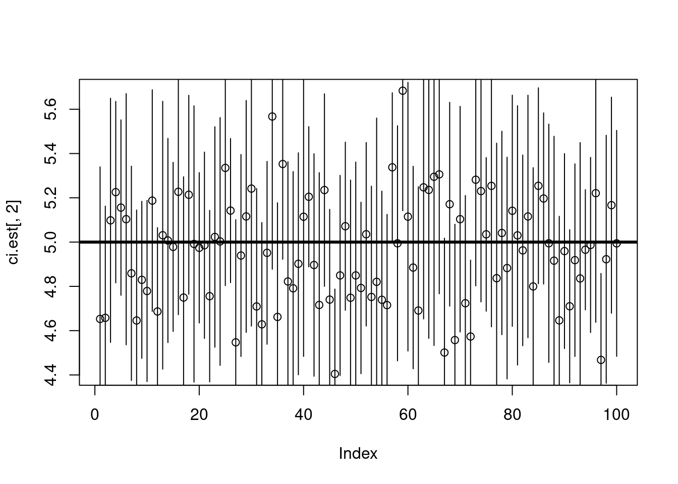
table(true_mean>ci.est[,1] & true_mean<ci.est[,3])
FALSE  TRUE
5 95 In frequentist, or parametric, statistics we assume that there is some true parameter value in the world. The data we observe are randomly drawn from distributions governed by those true parameters. We are the ones observing the truth imperfectly. We are trying to get at the ‘truth’ by taking a sample and making inference about the population based on our sample.
This concept also extends beyond simple things like a population mean, where we are basically fitting an intercept-only model where the intercept is the mean. It applies to all our parameter estimates. 95% of the time, if we went out and collected data and calculated parameter values in this way, we would end up capturing the ‘true’ parameter value.
It is very, very important to keep this distinction in mind because it is often reported incorrectly in the literature. A 95% confidence interval means that, 95% of the time if we do things this way, our estimate will contain the true population mean, and 5% of the time the true mean will fall outside our estimate. It does NOT mean that there is a 95% probability that the true value lies within that range. There is no probability associated with the true value. It is just some immutable thing, out there in the world, that we are trying to understand. If you want to actually be able to assign probabilities to parameter values, join me on the dark side and go Bayesian.
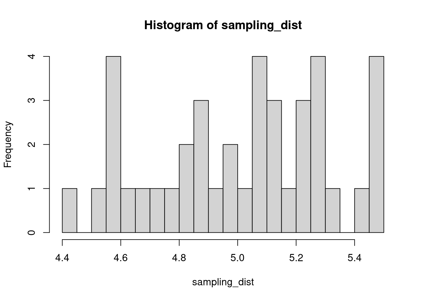
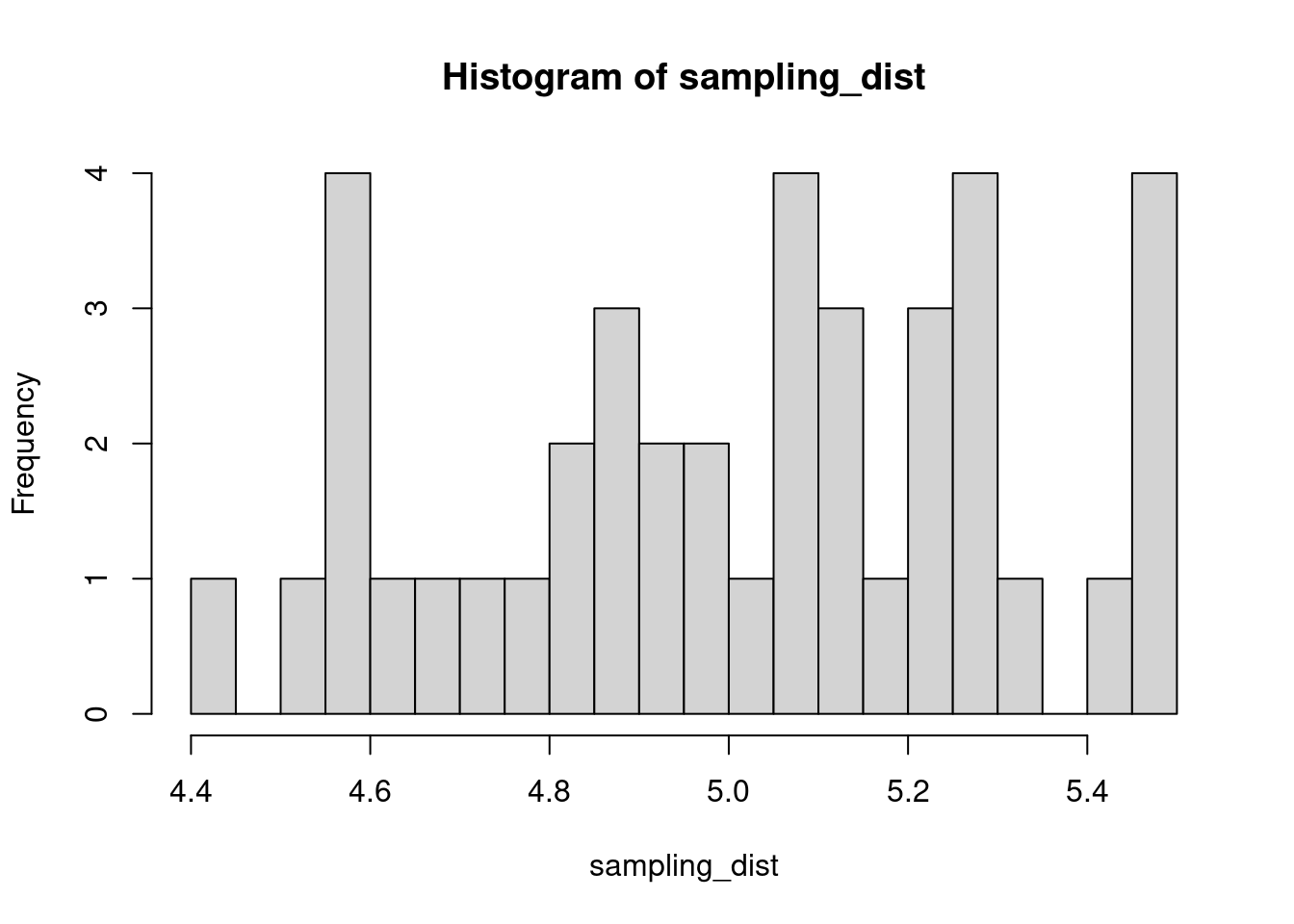
The sample distribution is quite literally just the distribution of values in our sample. So for example, in our salamander example, Joe’s sample distribution is the aggressiveness scores of the 15 salamanders he encountered. We could also generate something that is confusingly called the sampling distribution, which is the distribution of some metric calculated on our sample distribution(s). Because we could send out let’s say 100 BIOL 431 students, each time we send someone out we could calculate the mean of their sample. As our sample size approaches infinity, the sampling distribution will become increasingly normal shaped and the mean of the sampling distribution will approximate the true population mean.
sampling_dist <- c()

for(i in 1:100){
  student <- rnorm(sample_N, true_mean, true_sd)
  sampling_dist[i] <- mean(student)
  hist(sampling_dist, 20)
}
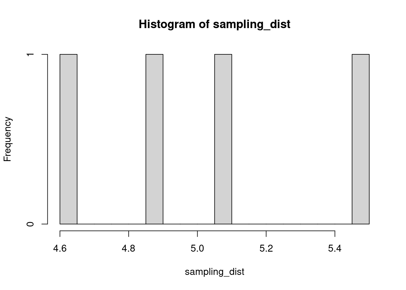
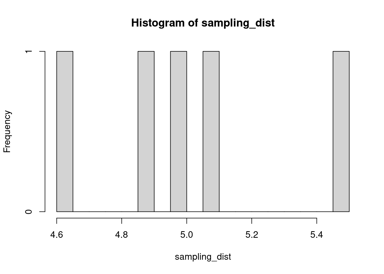
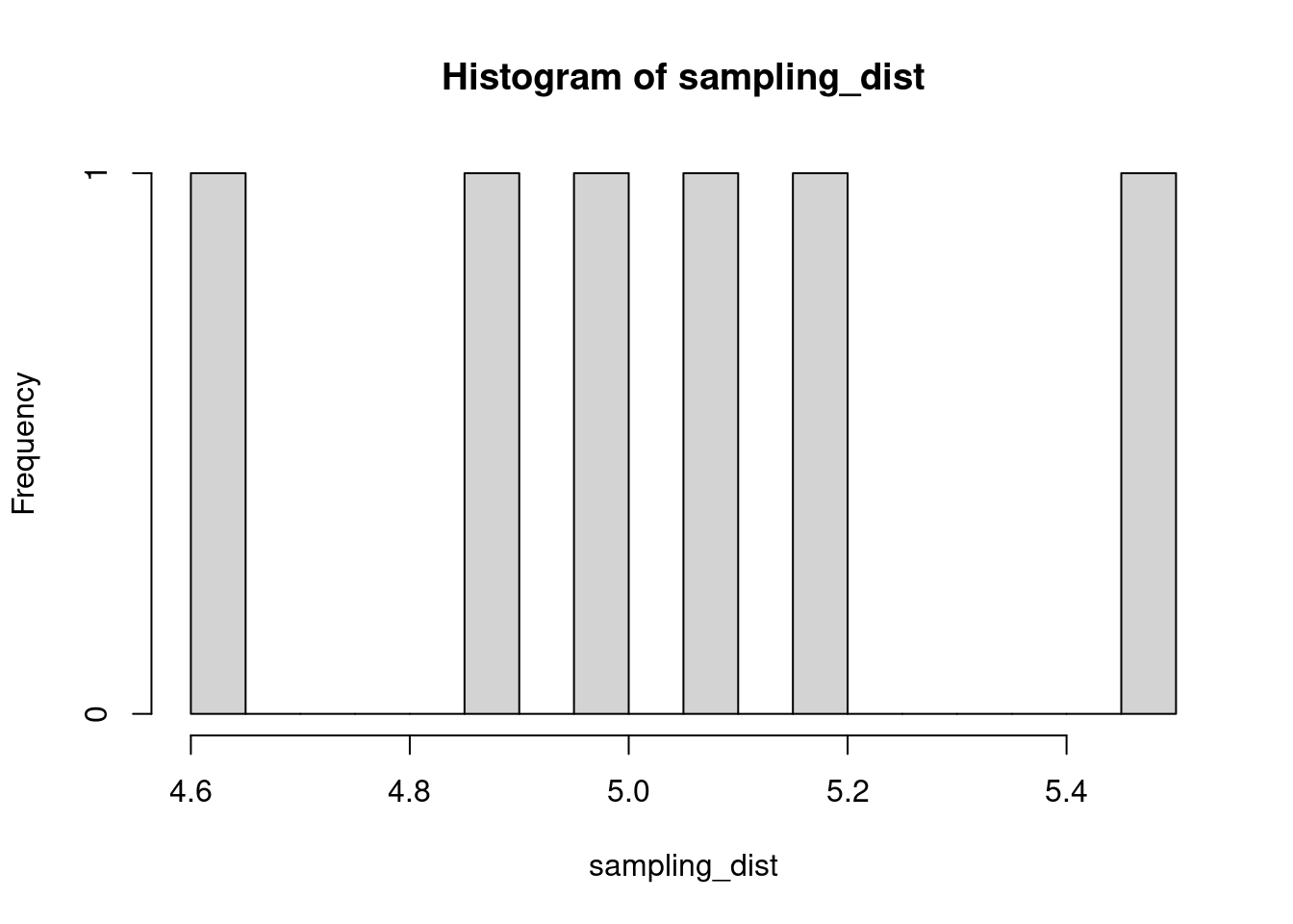
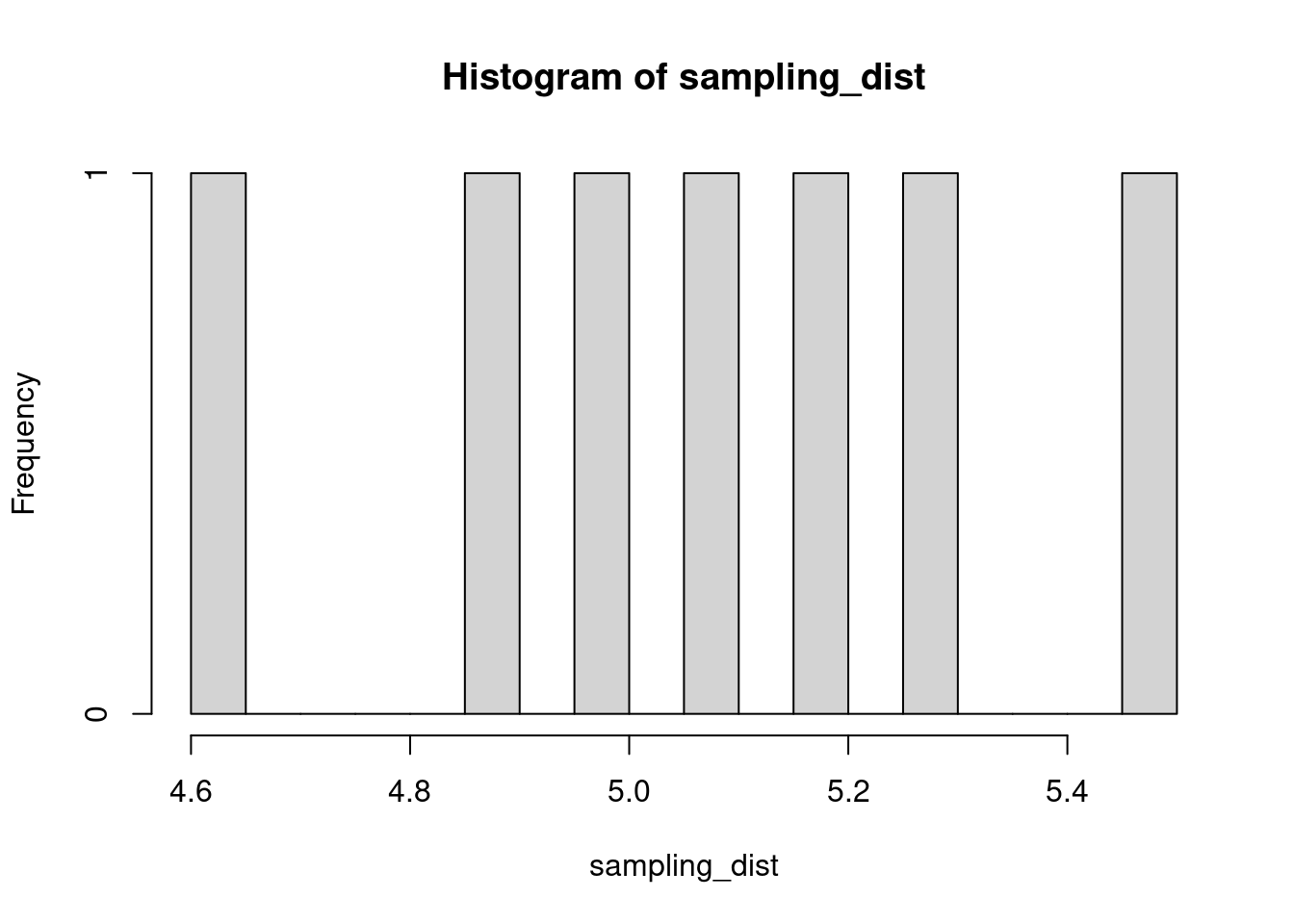
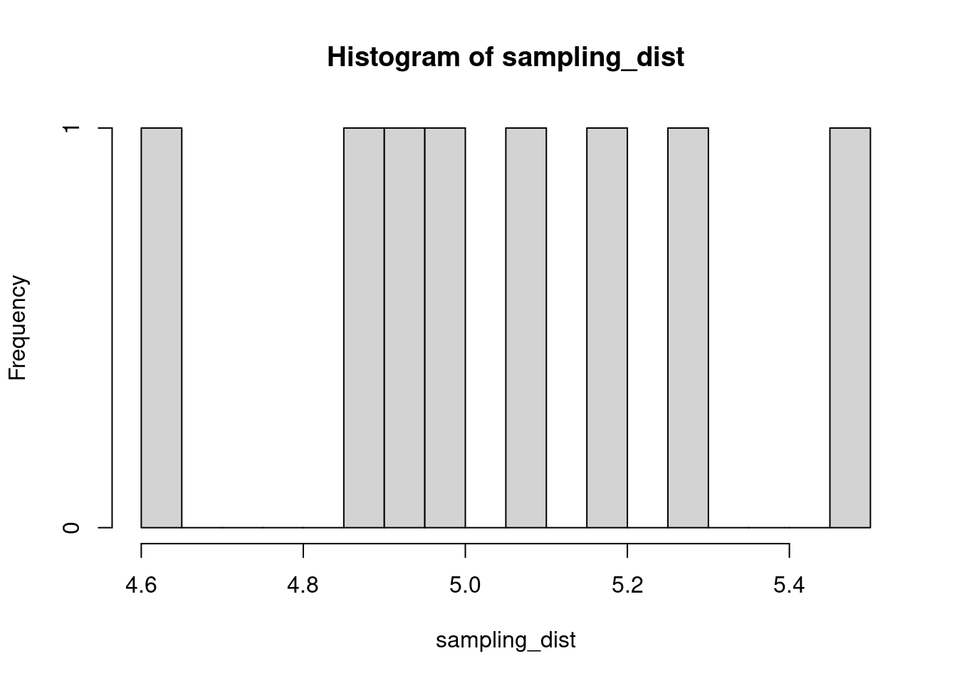
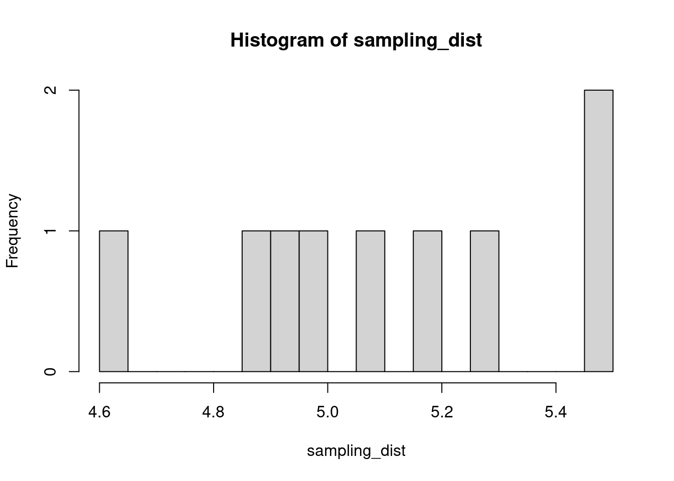
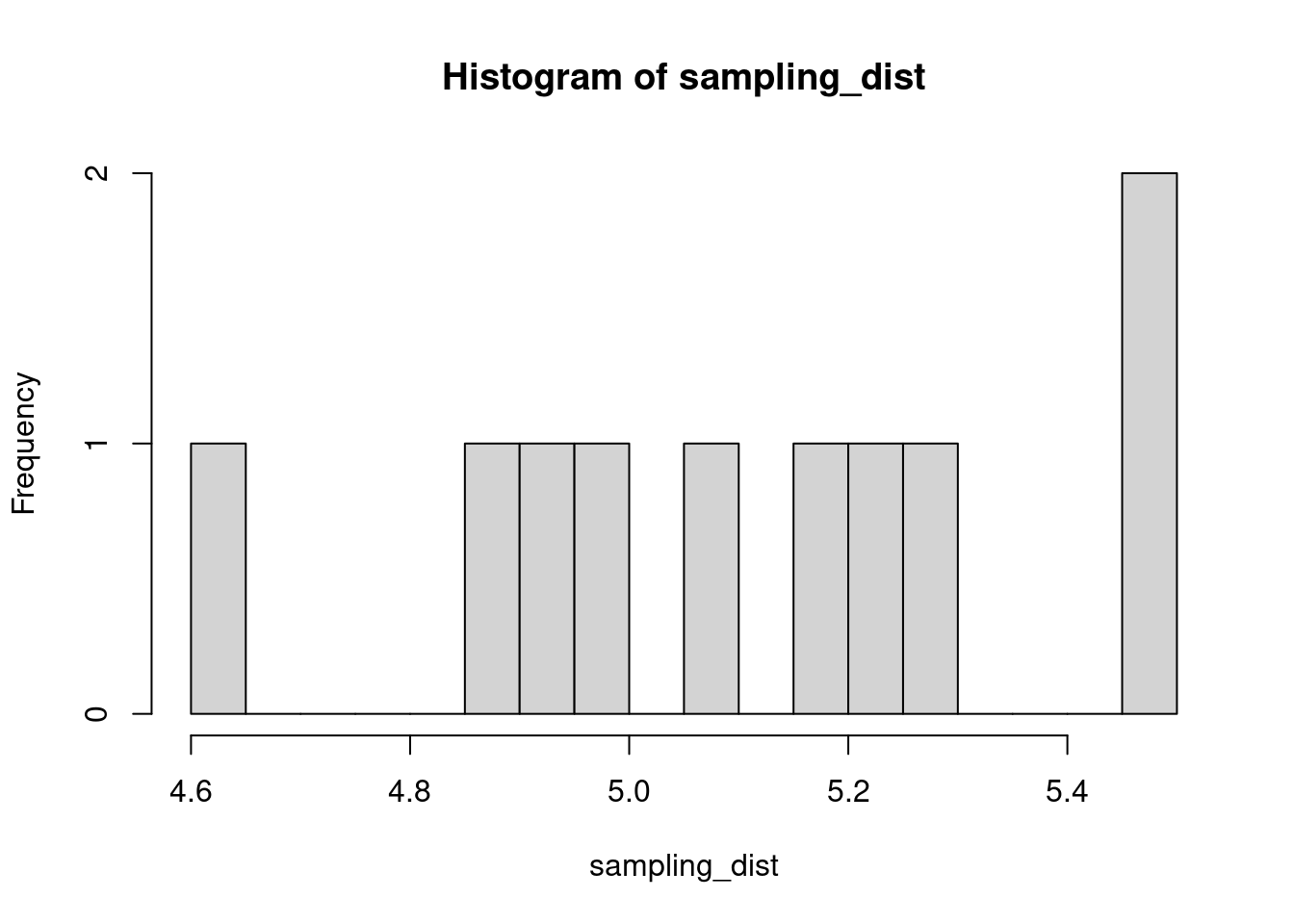
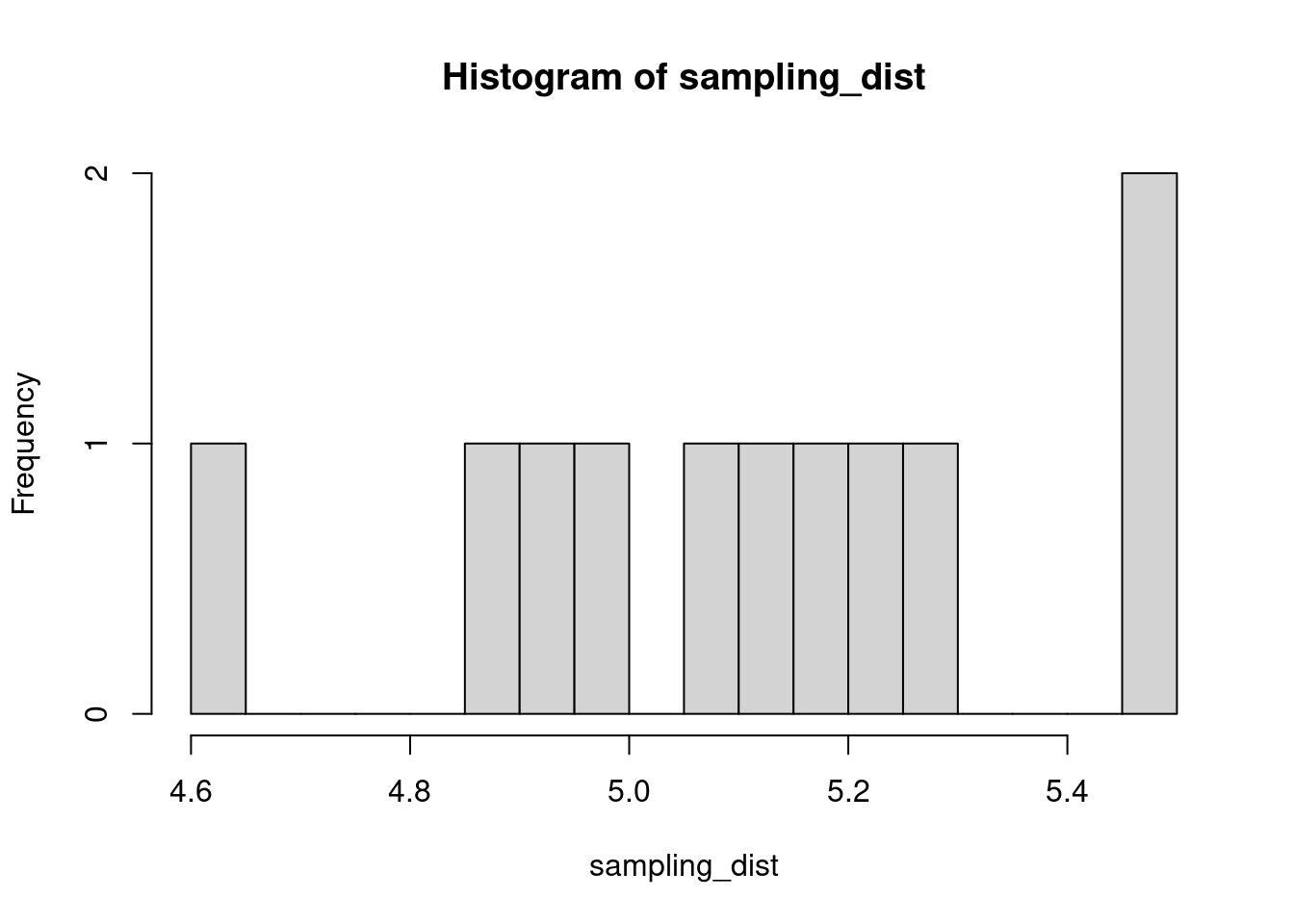
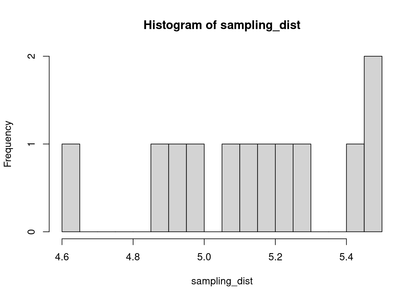
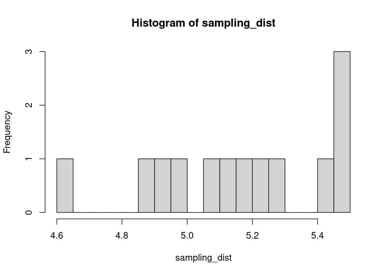
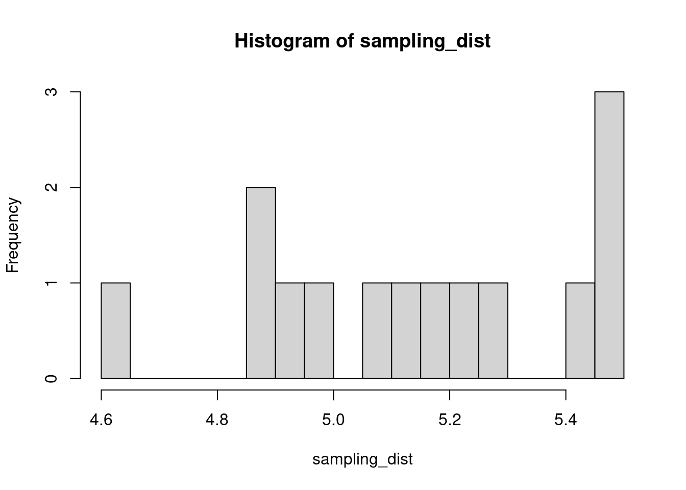
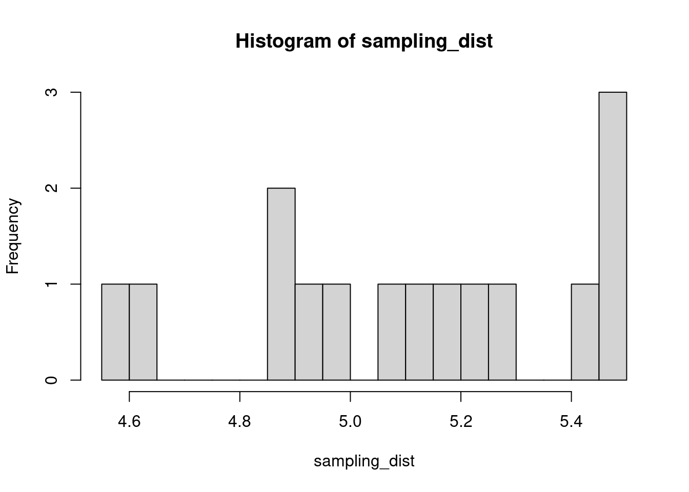
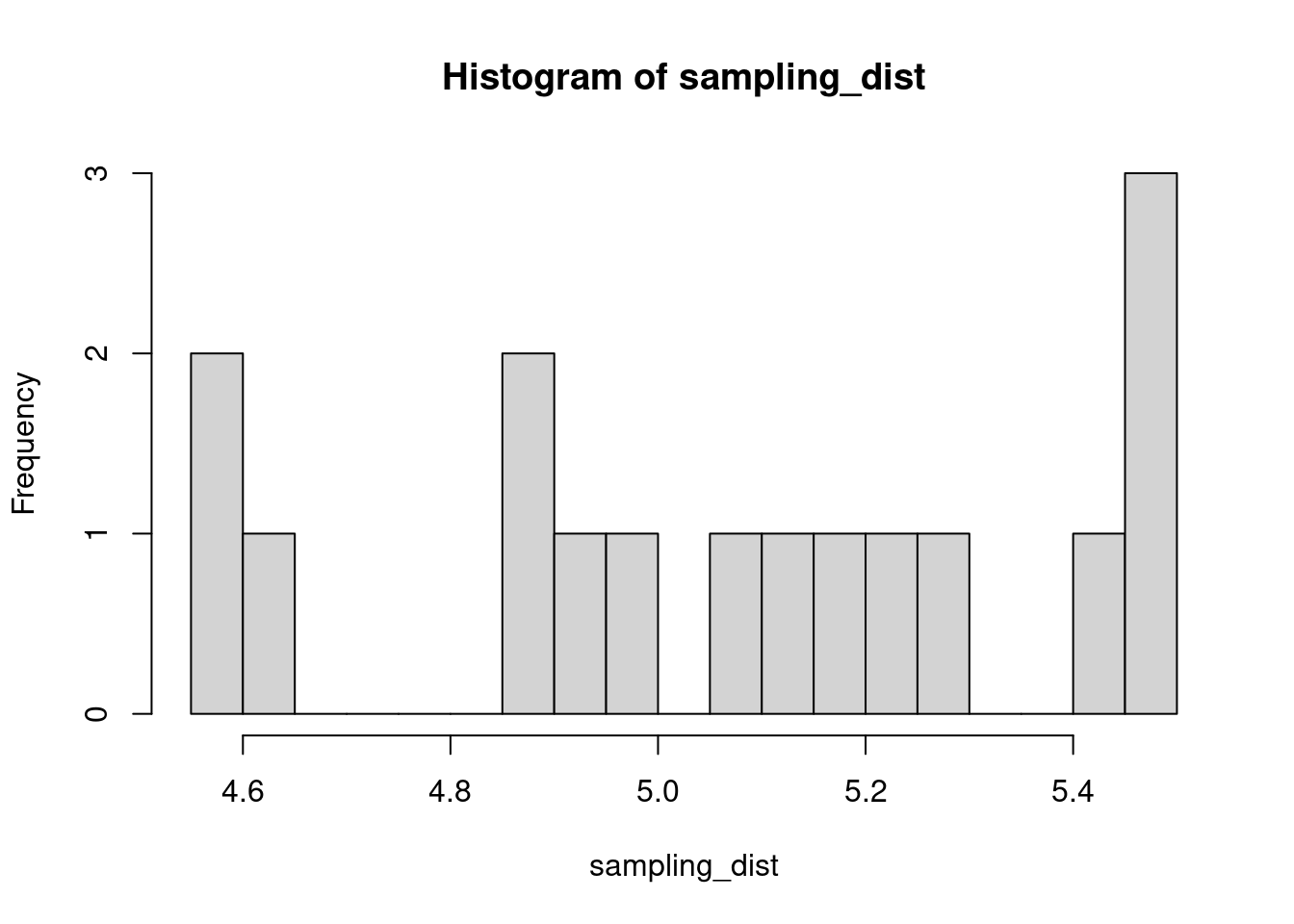
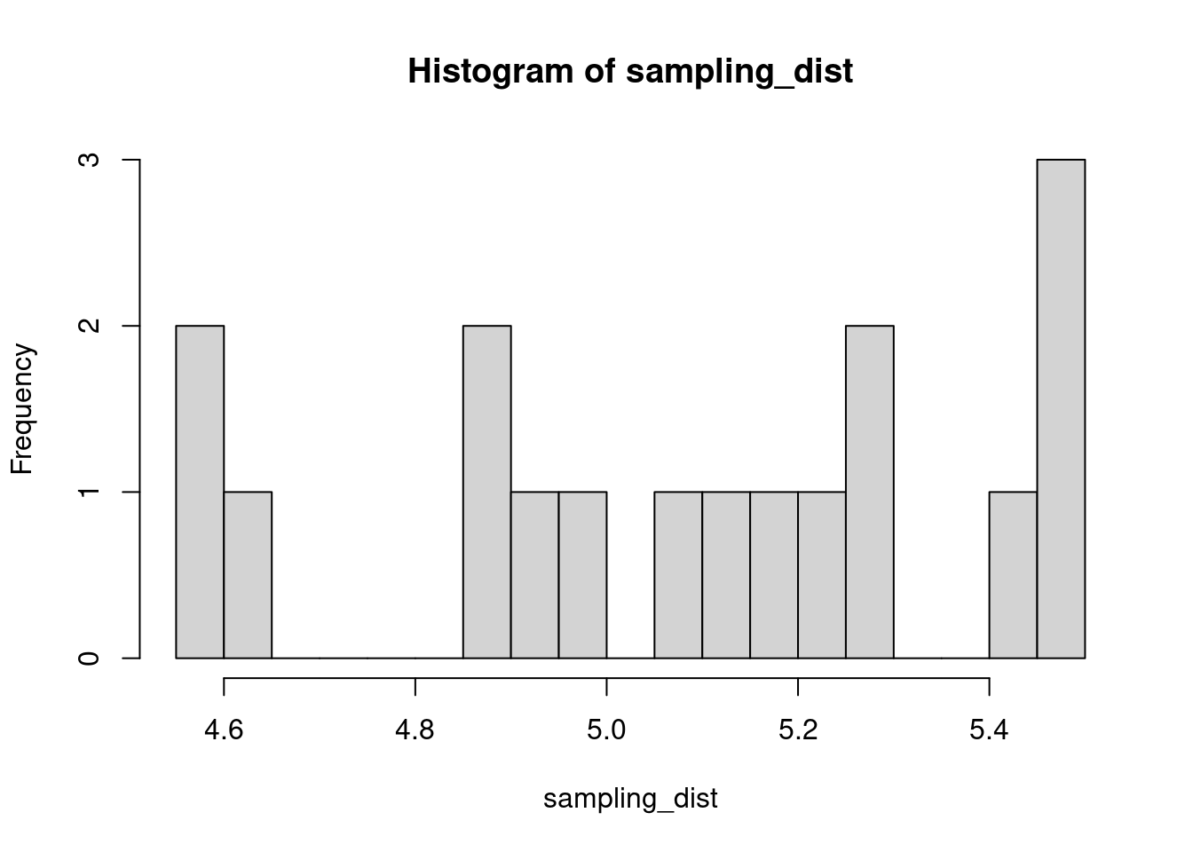
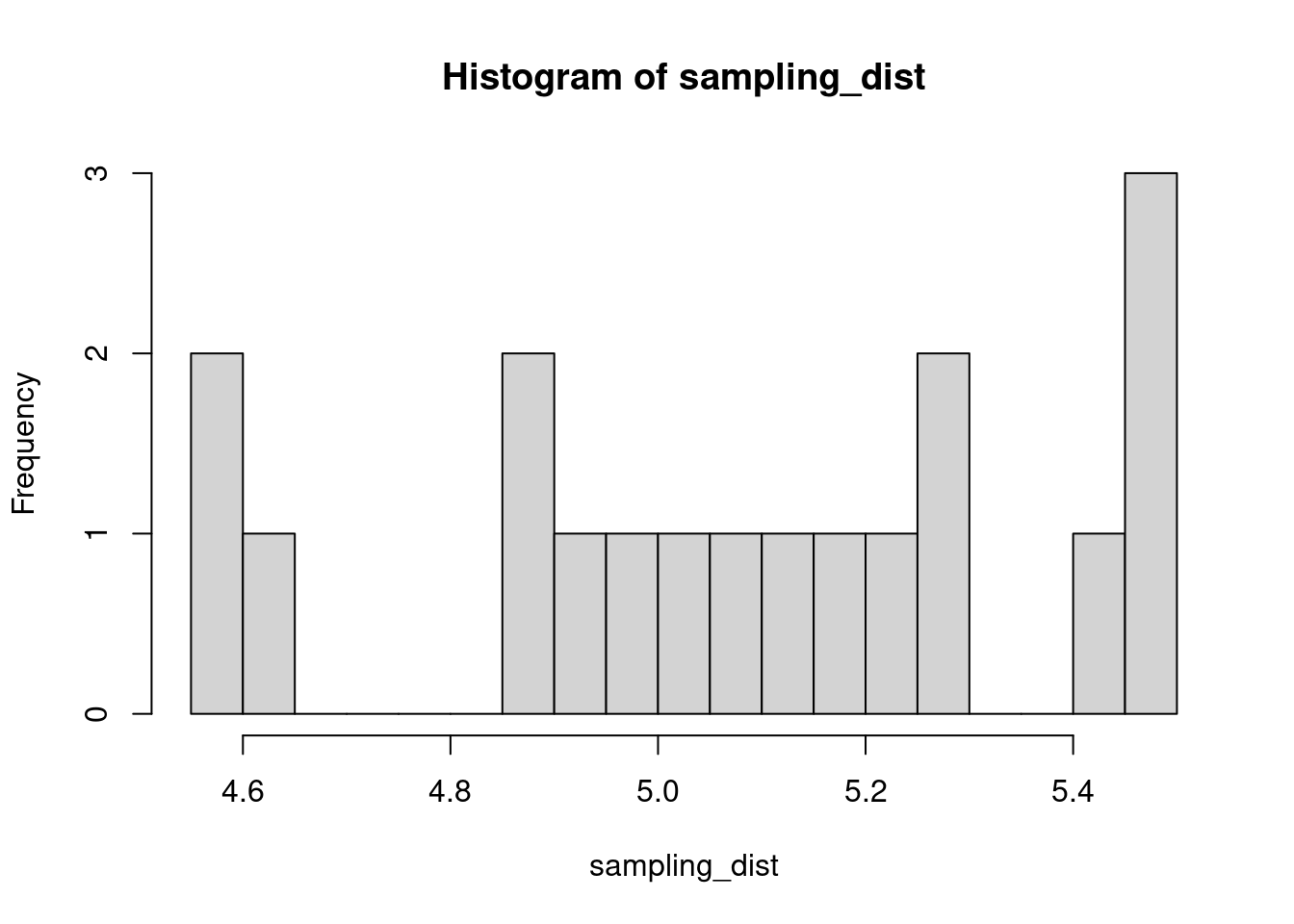
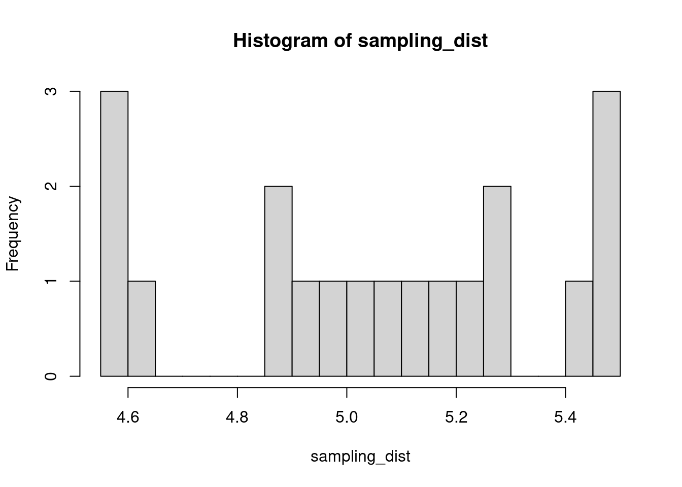
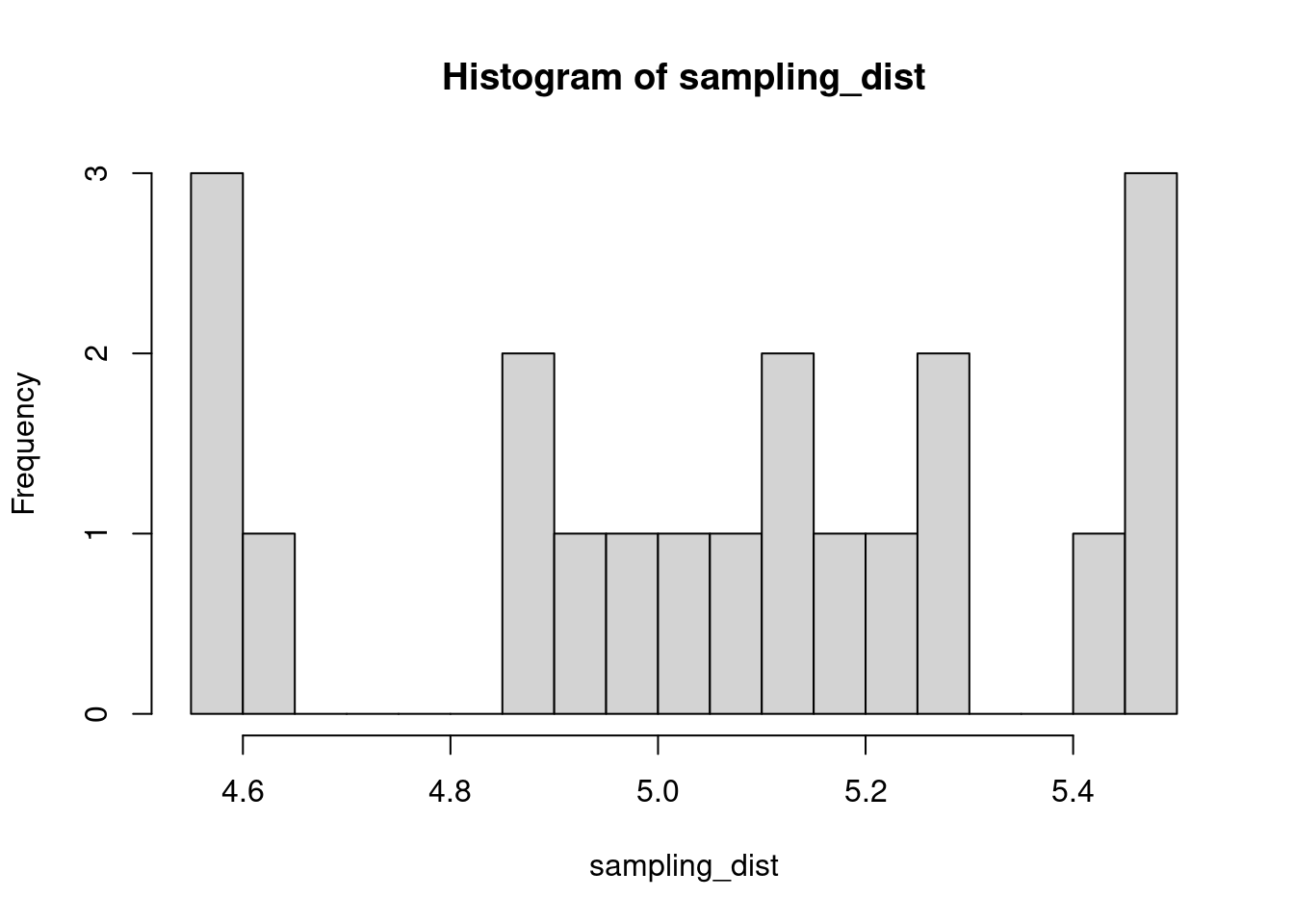
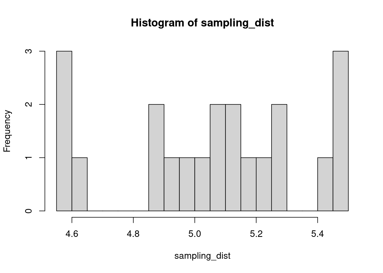
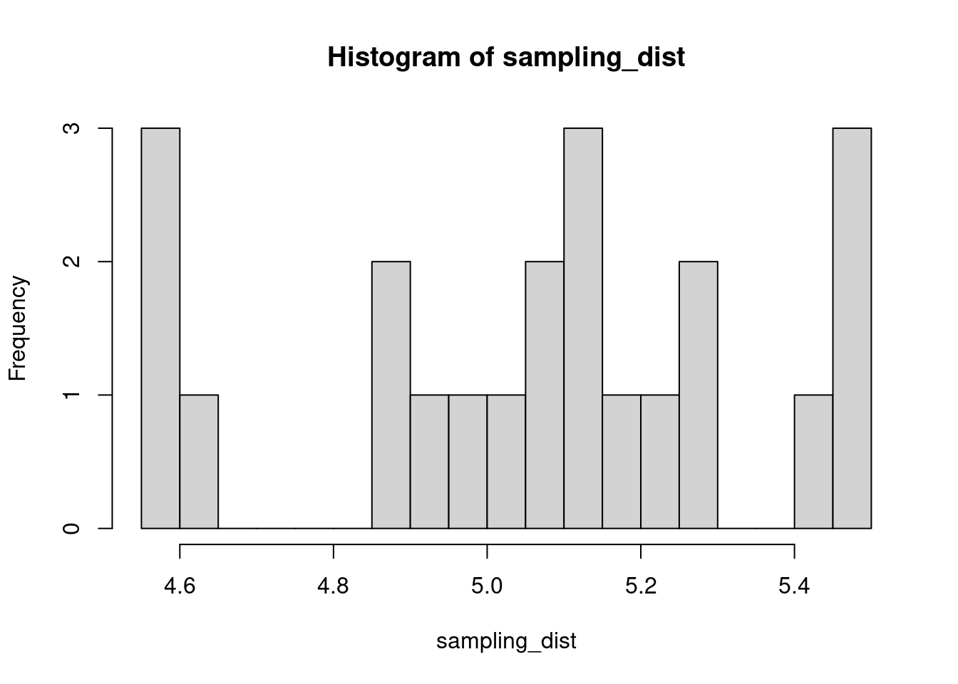
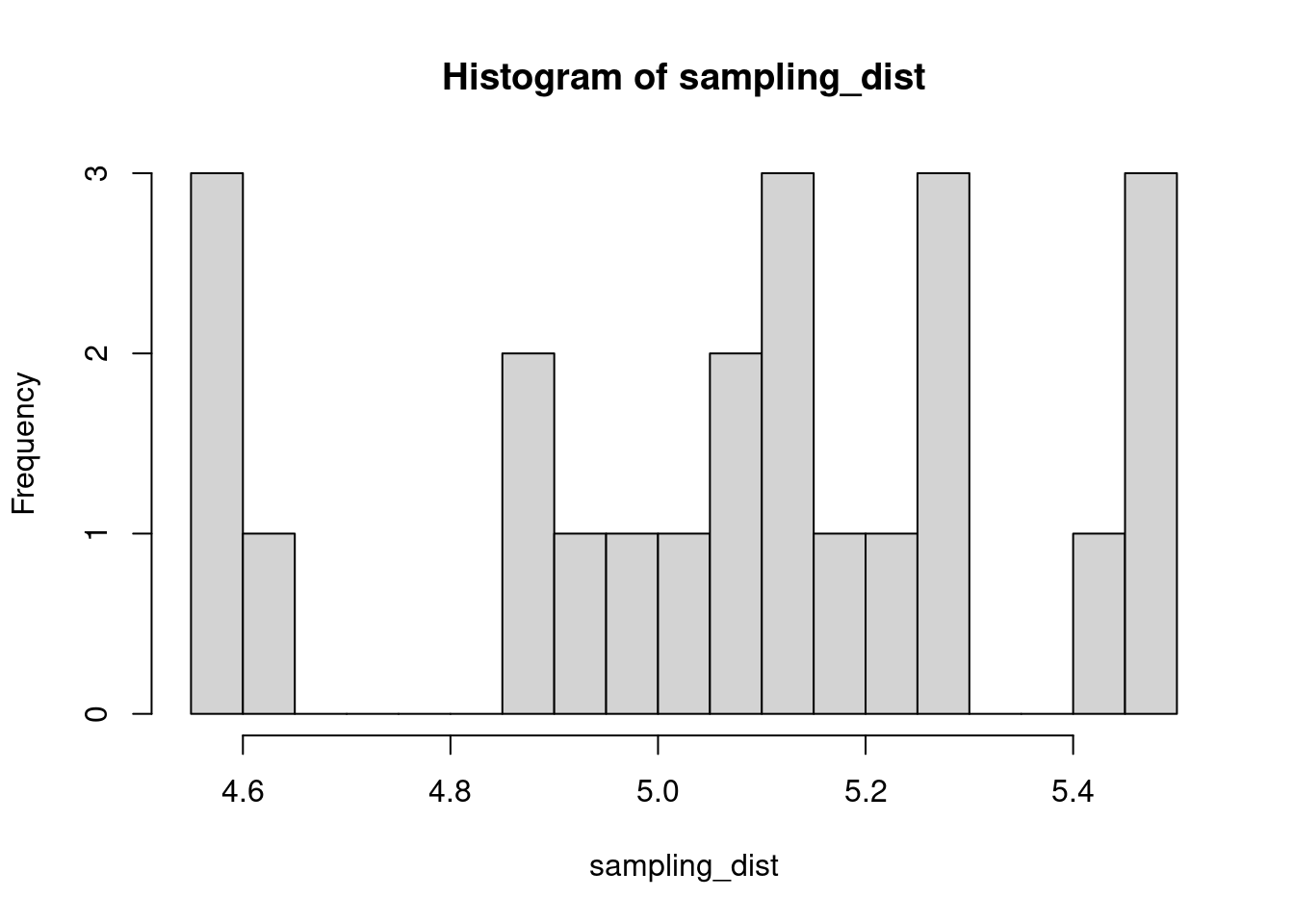
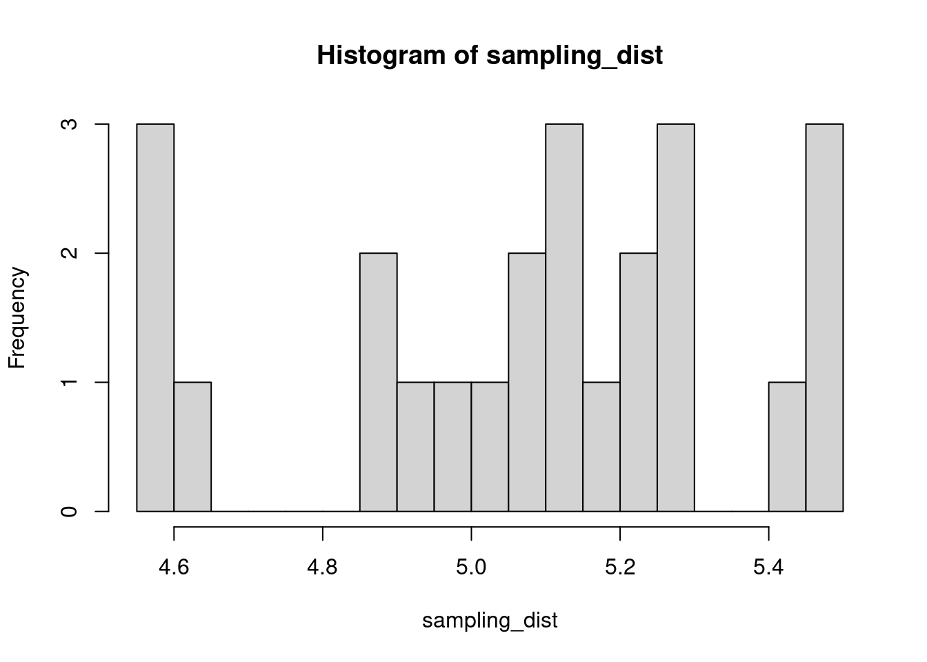
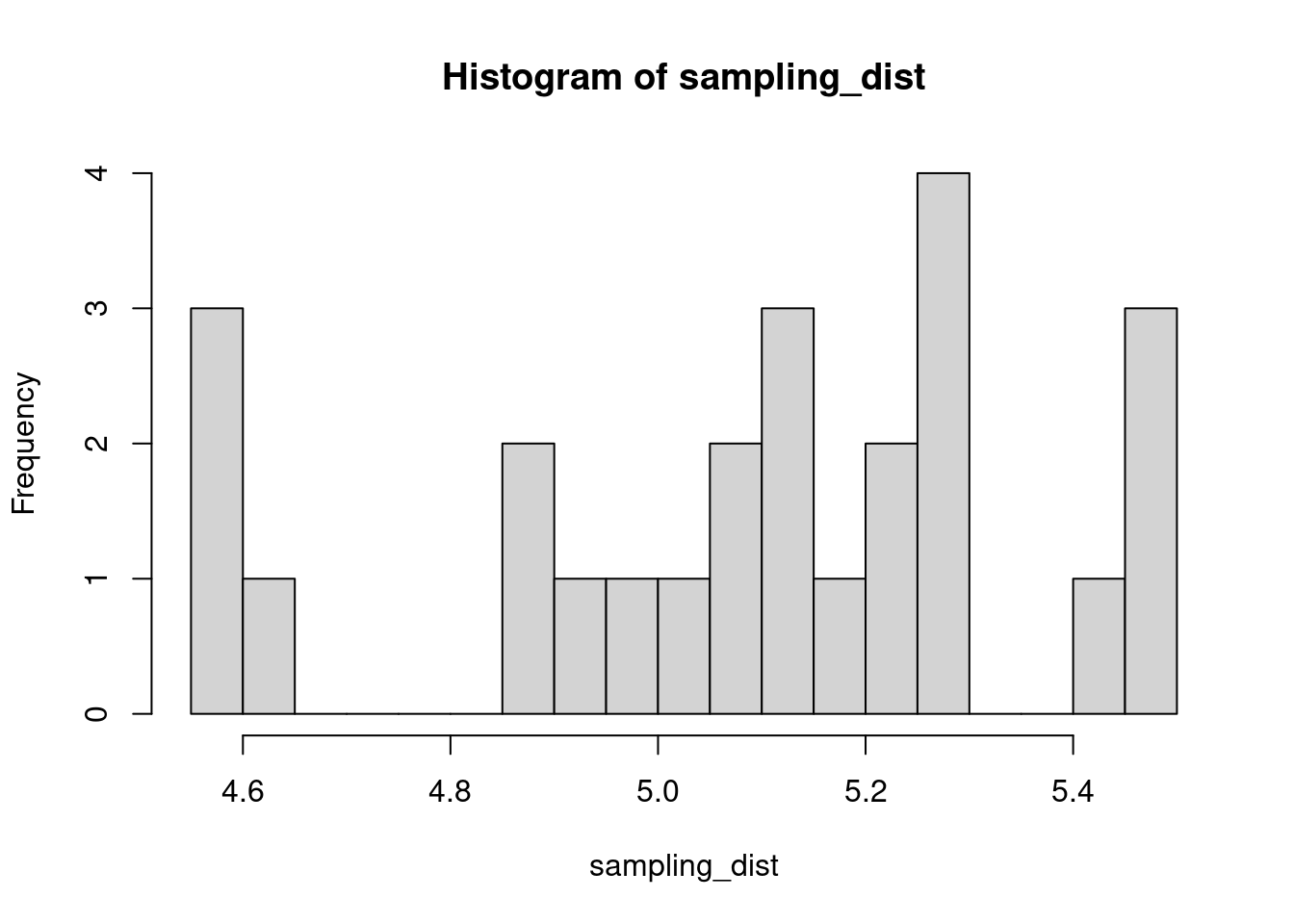
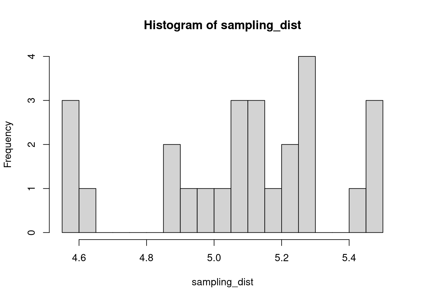
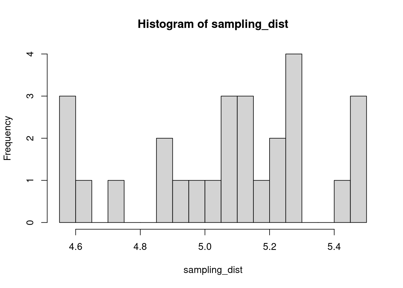
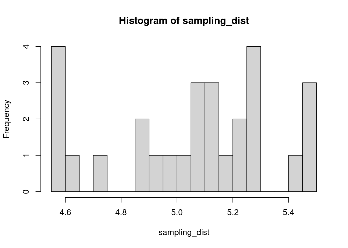
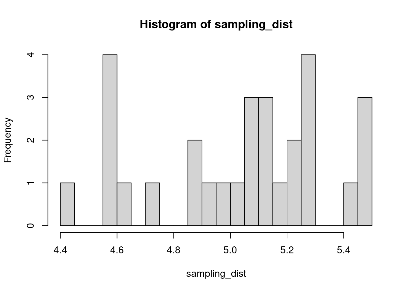
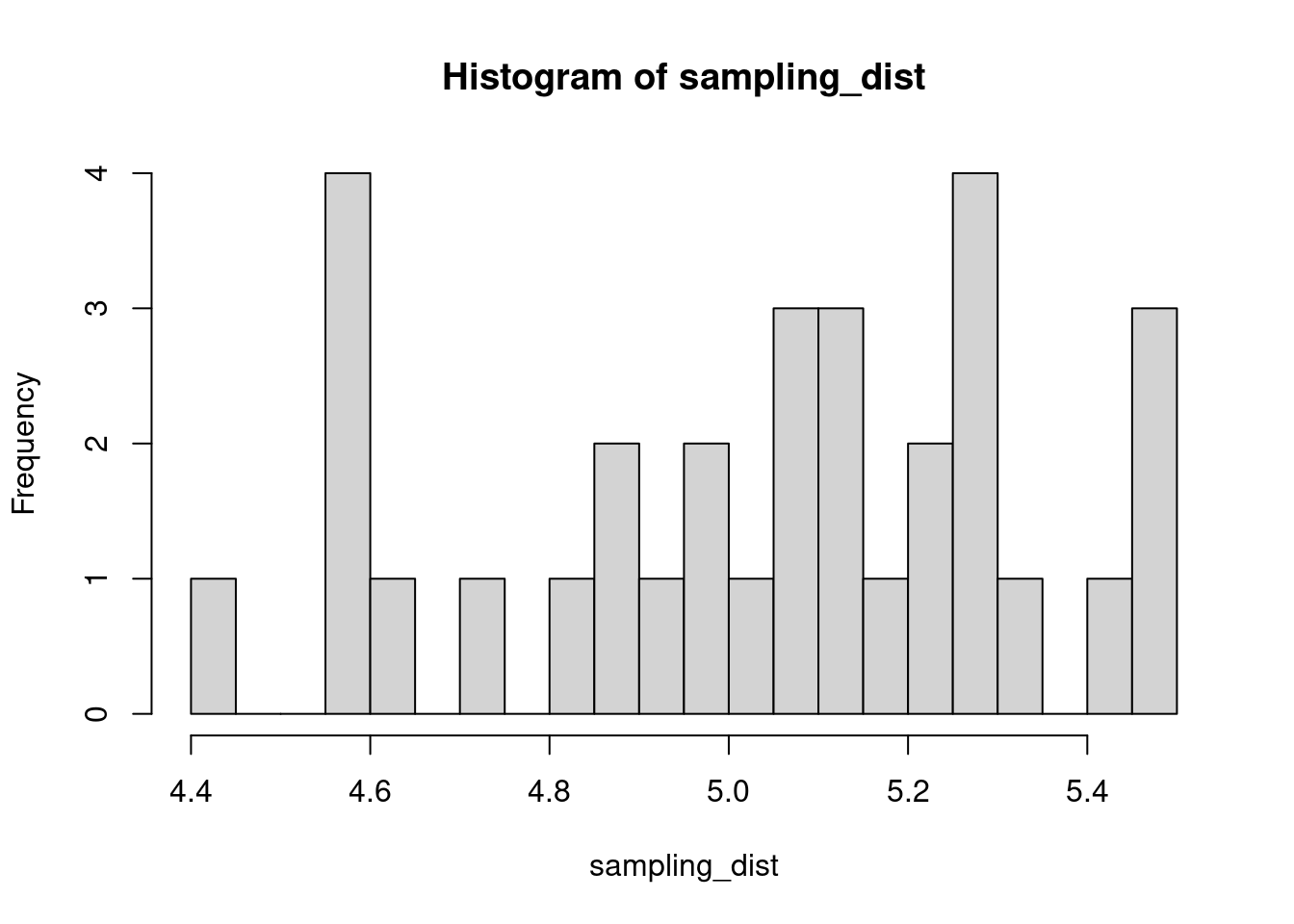
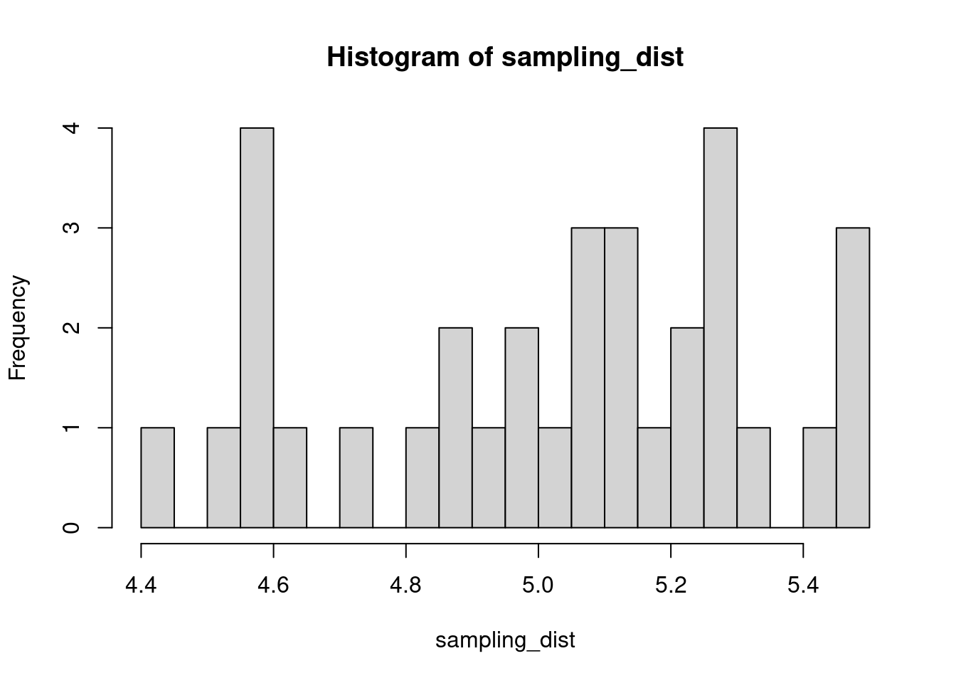
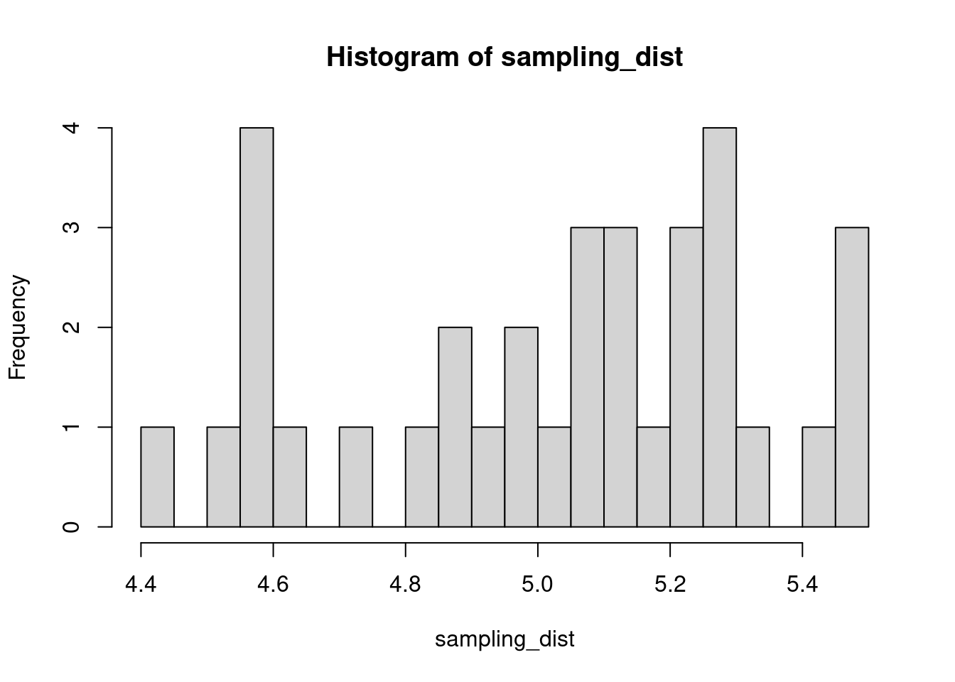
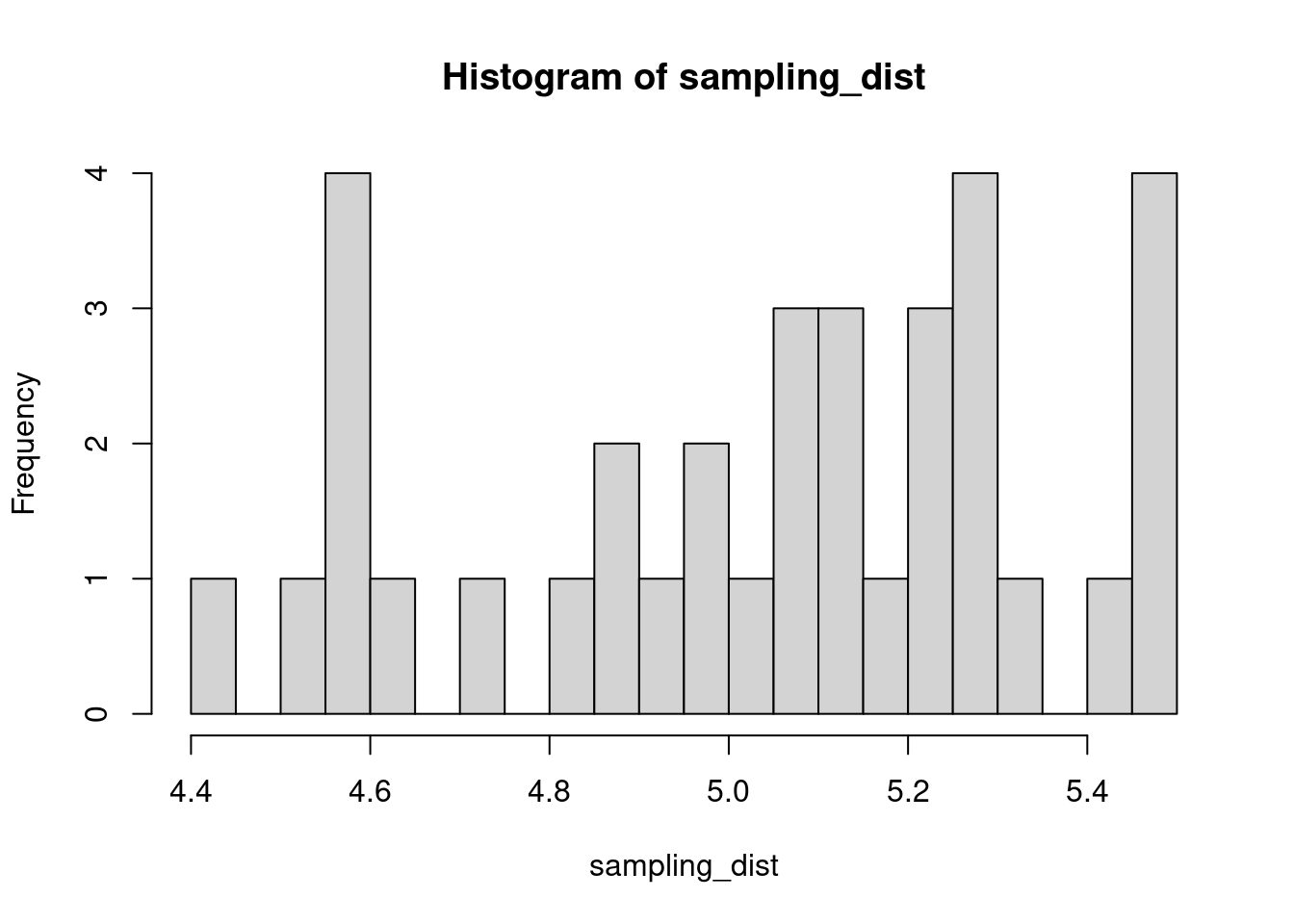
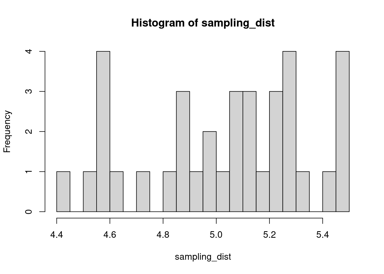
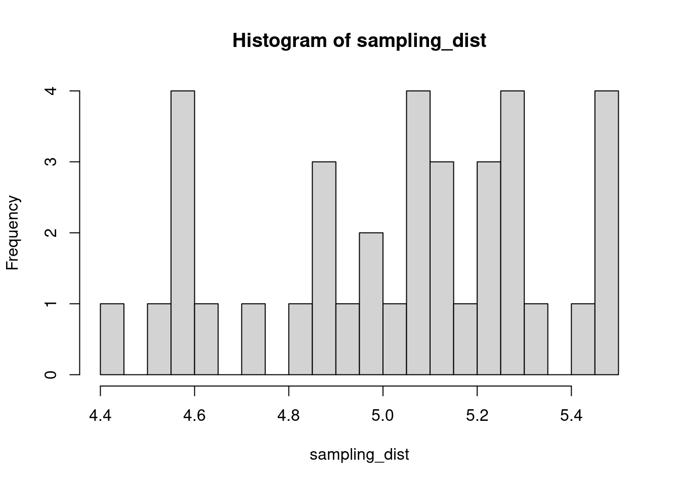
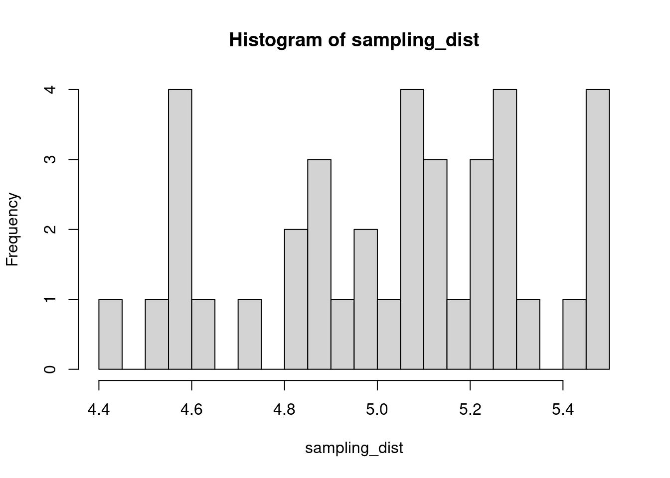
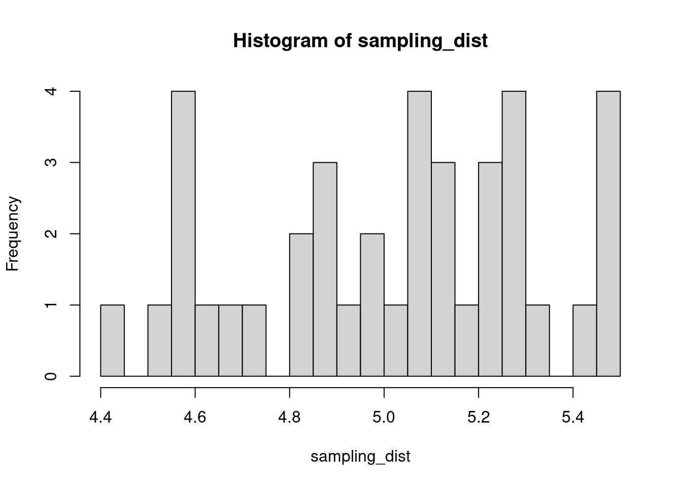
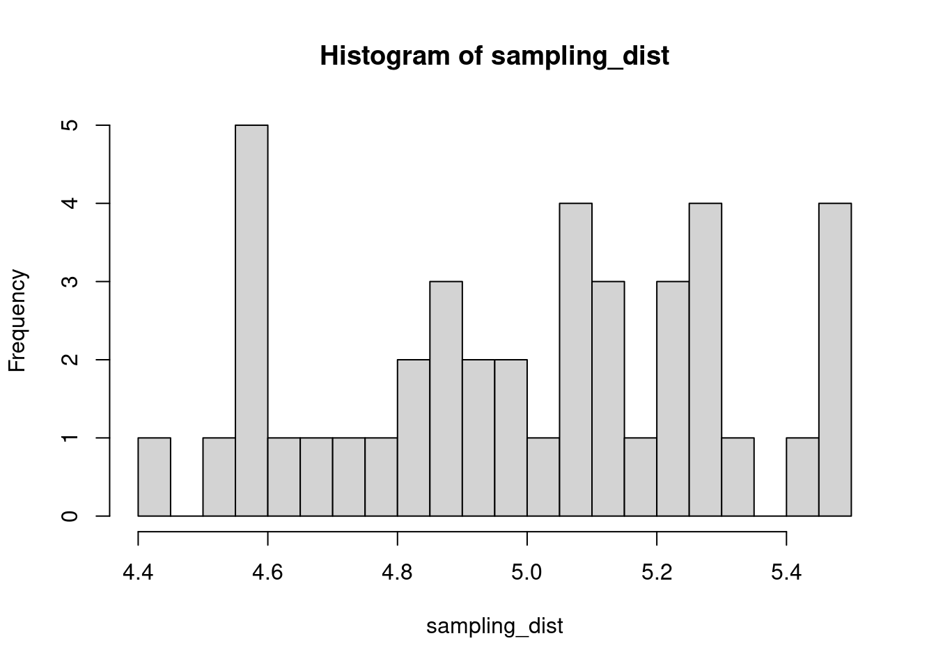
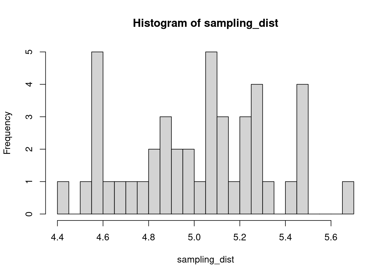
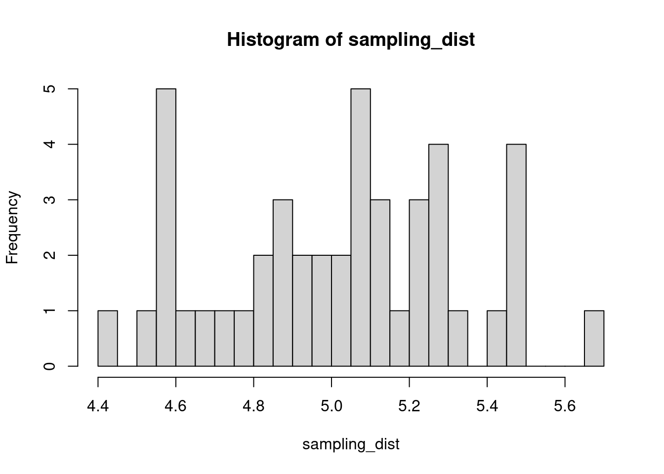
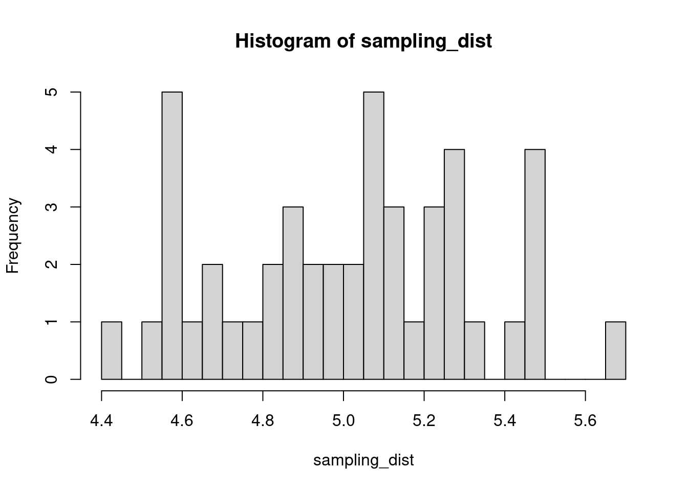
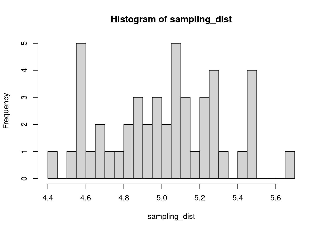
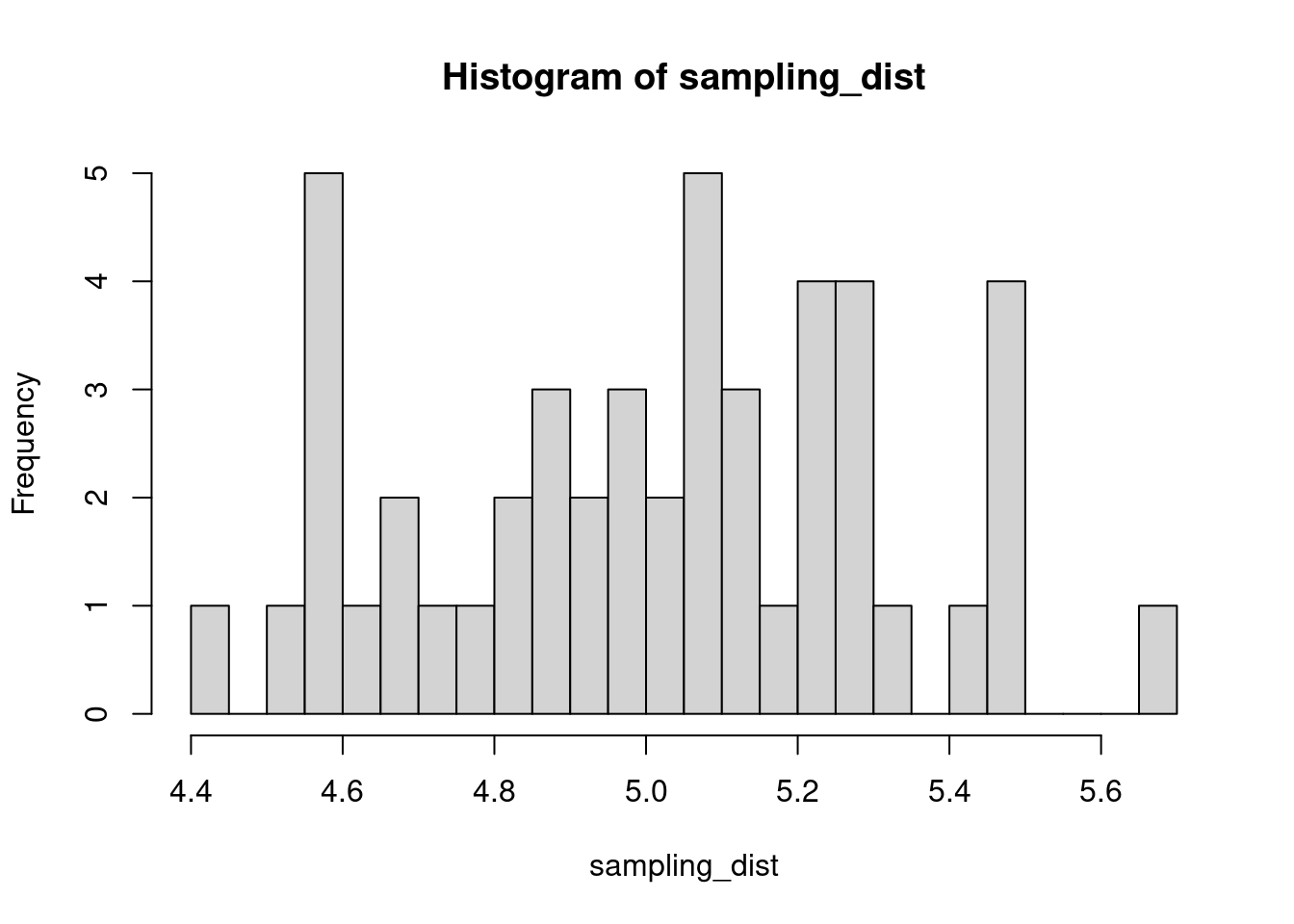
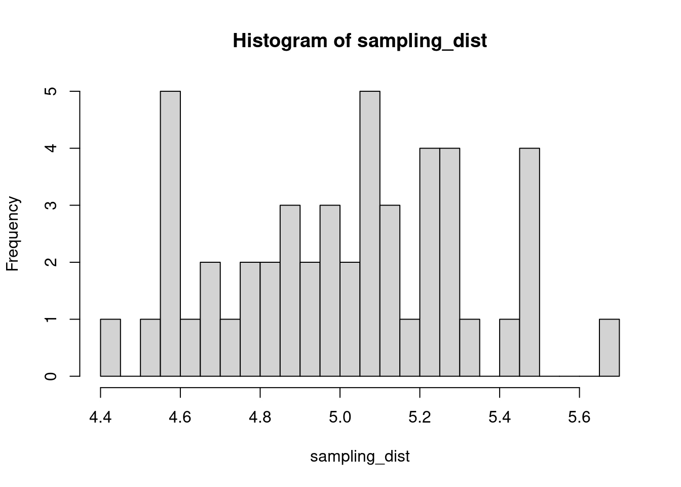
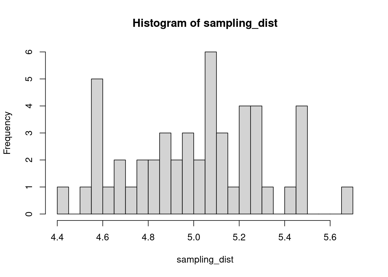
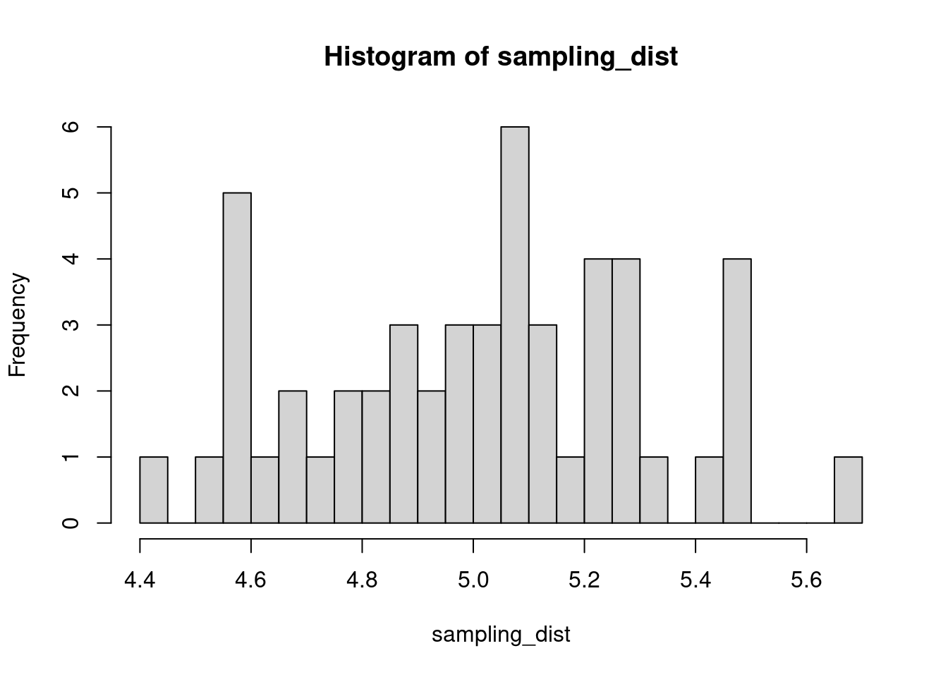
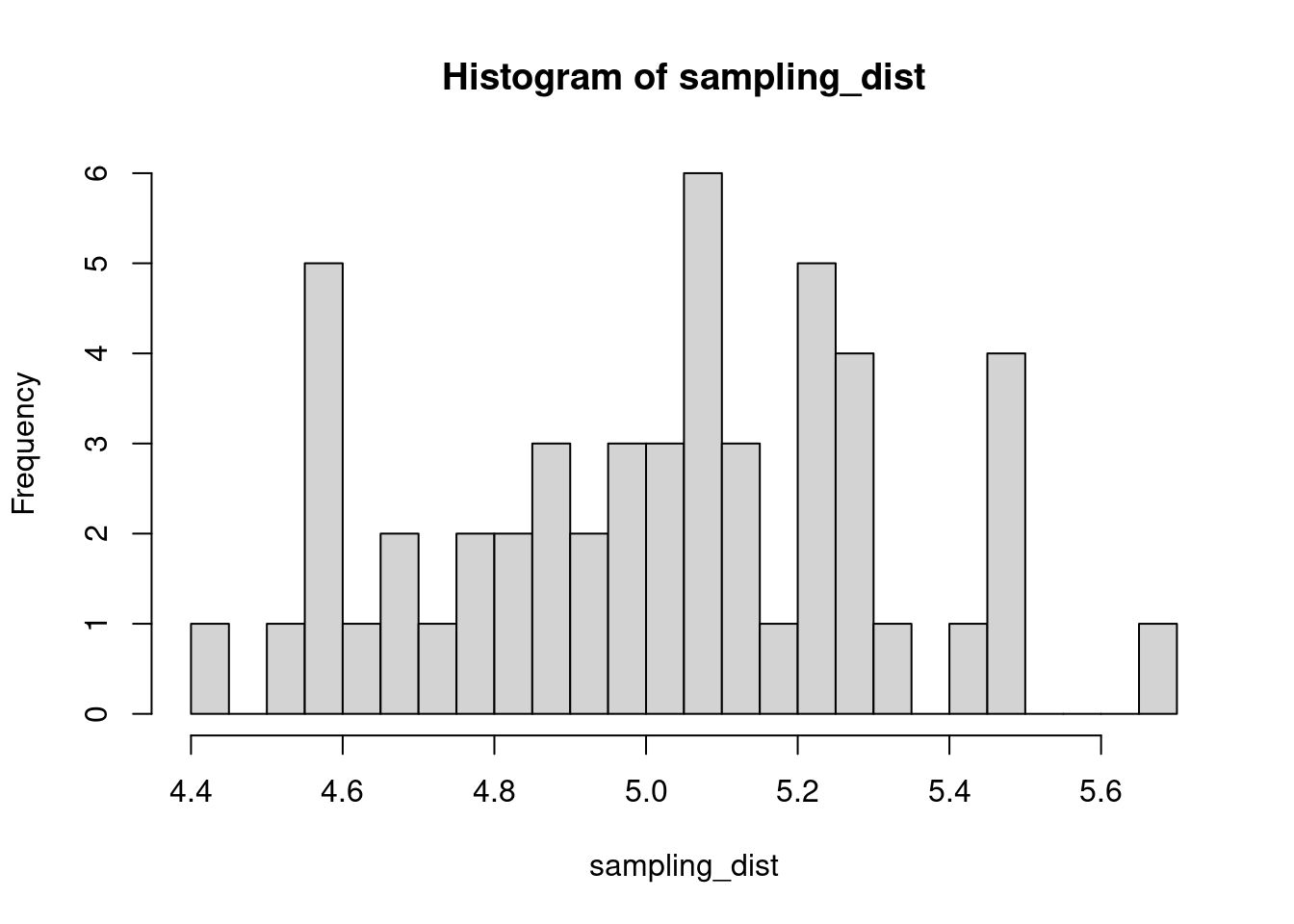
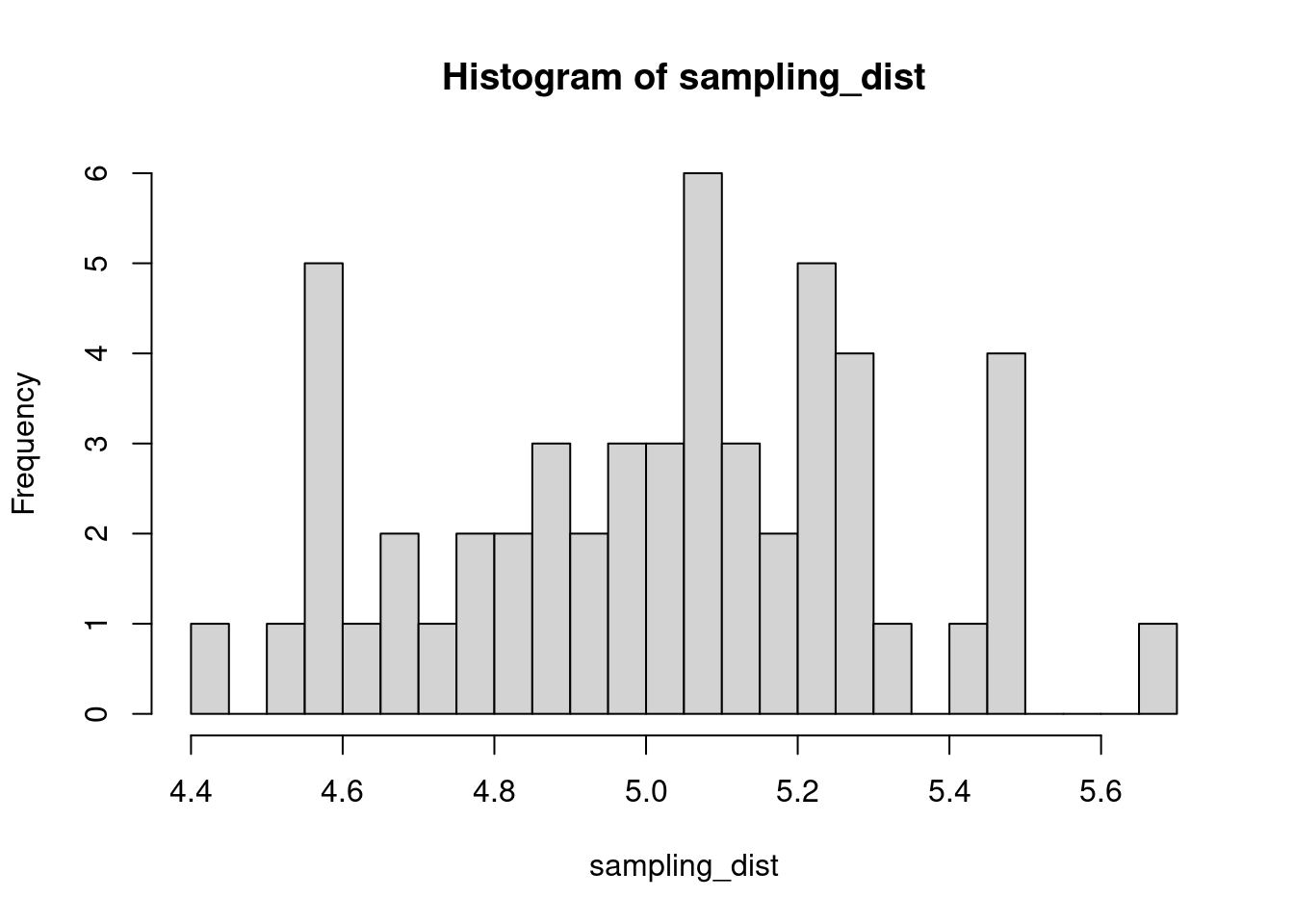
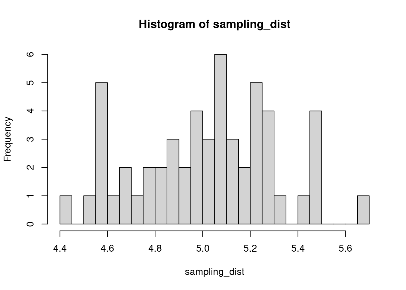
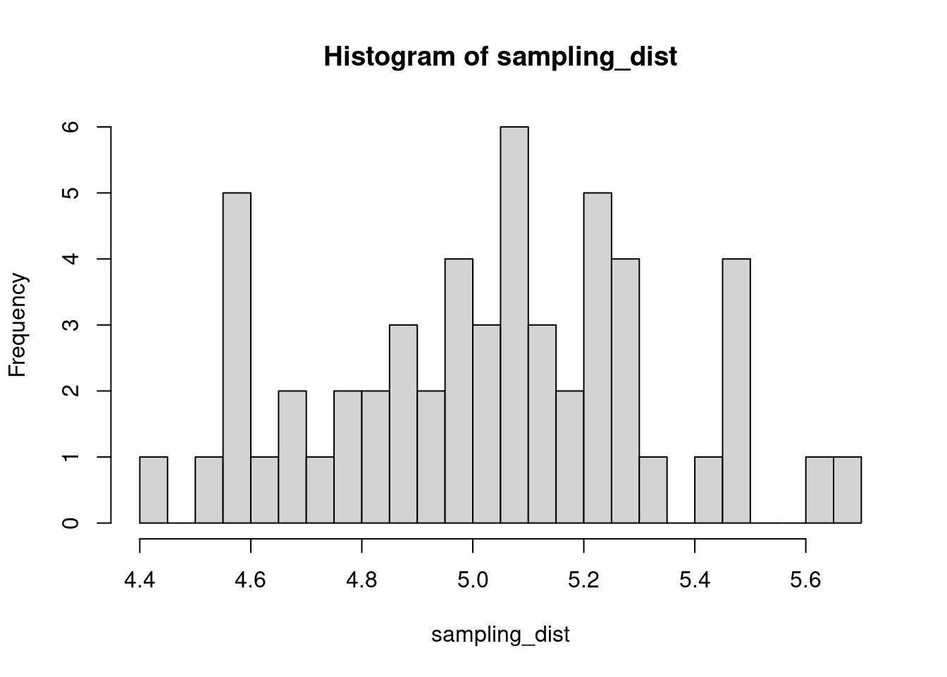
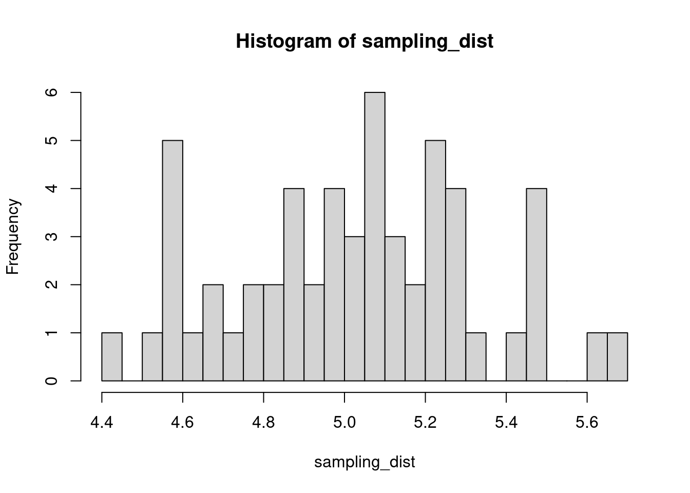
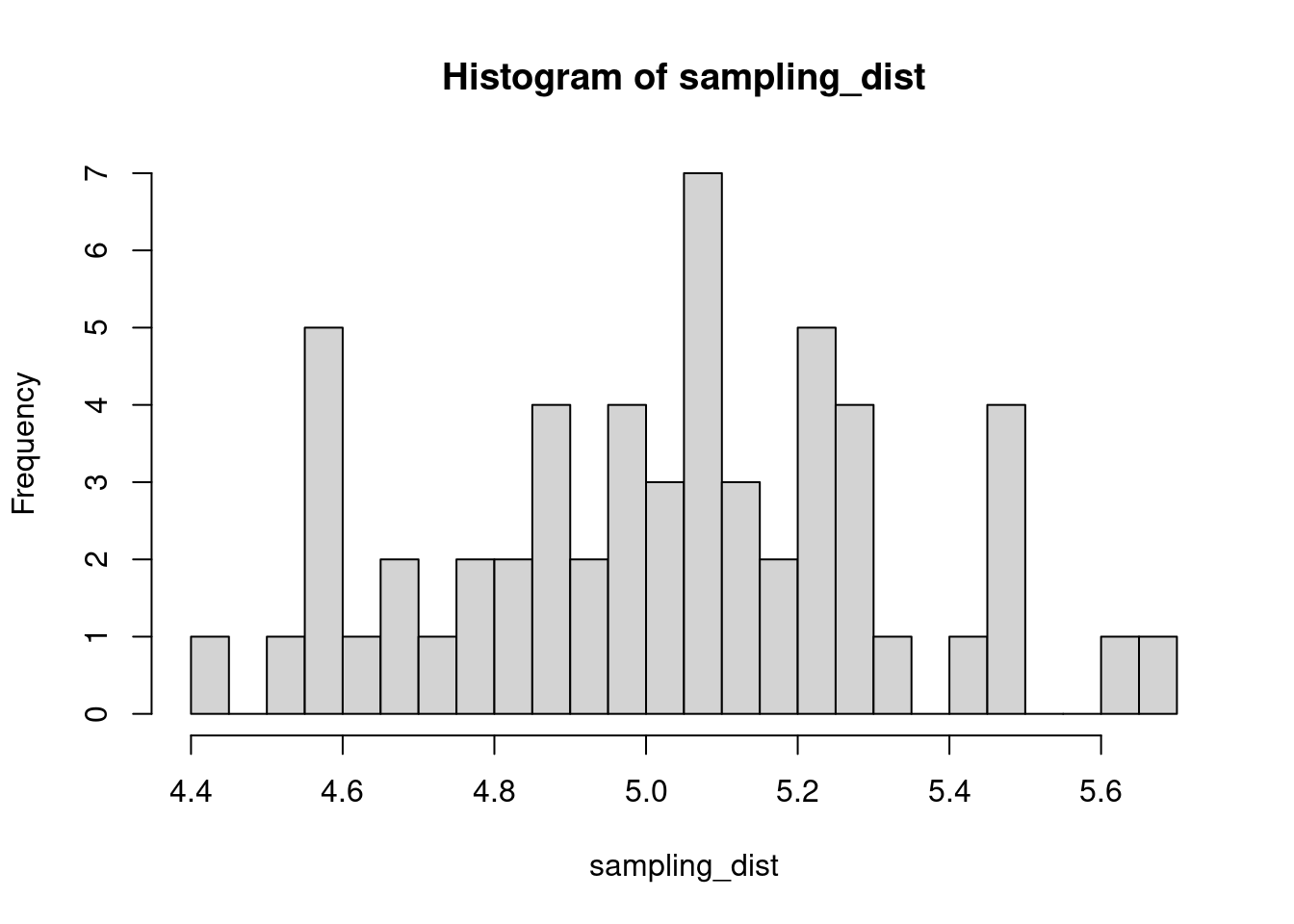
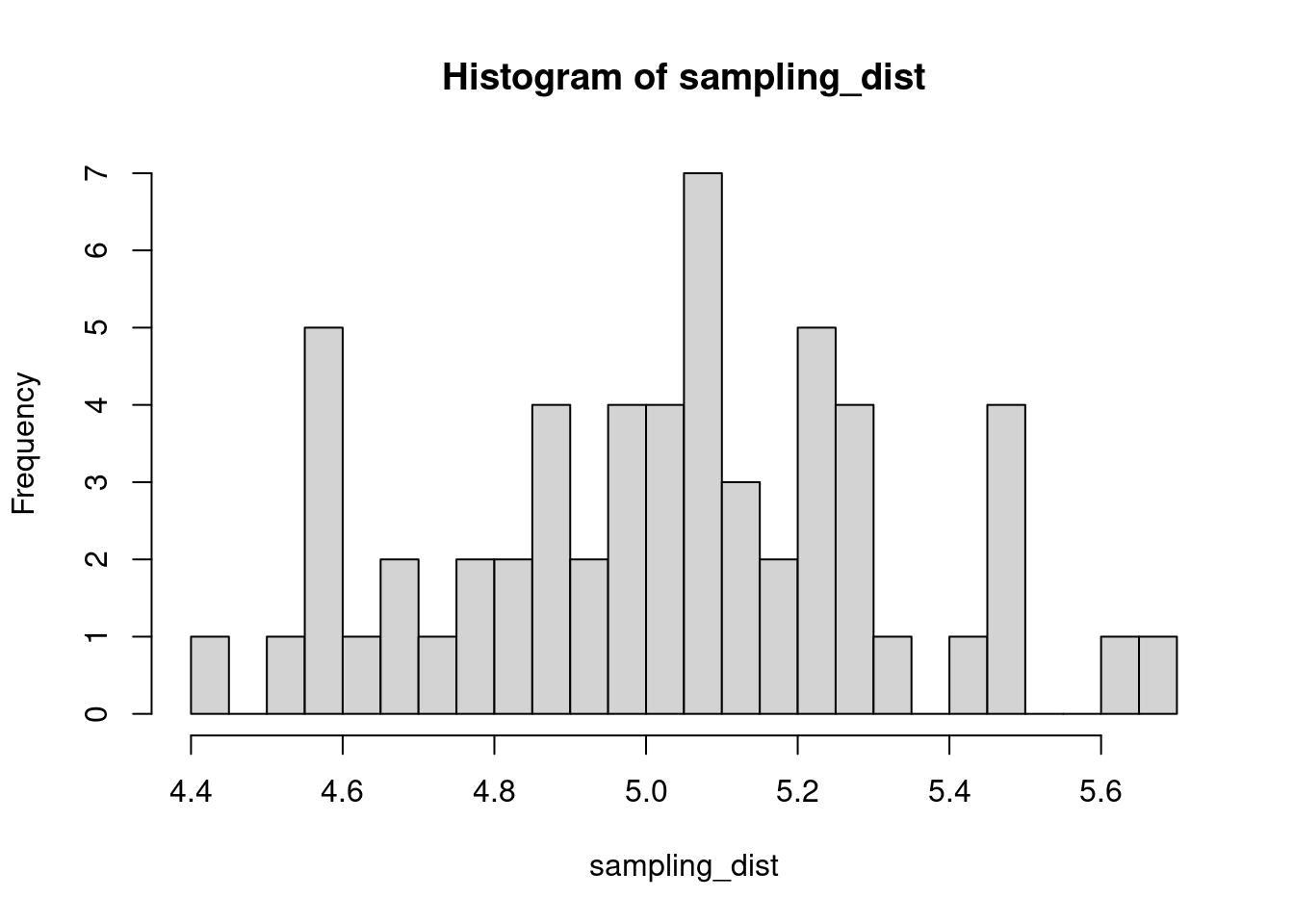
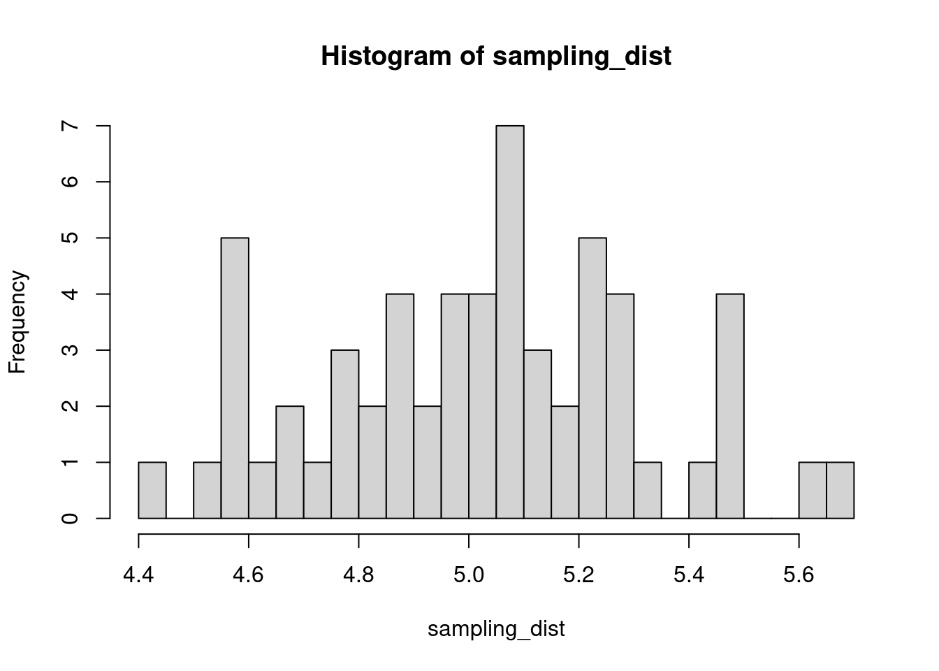
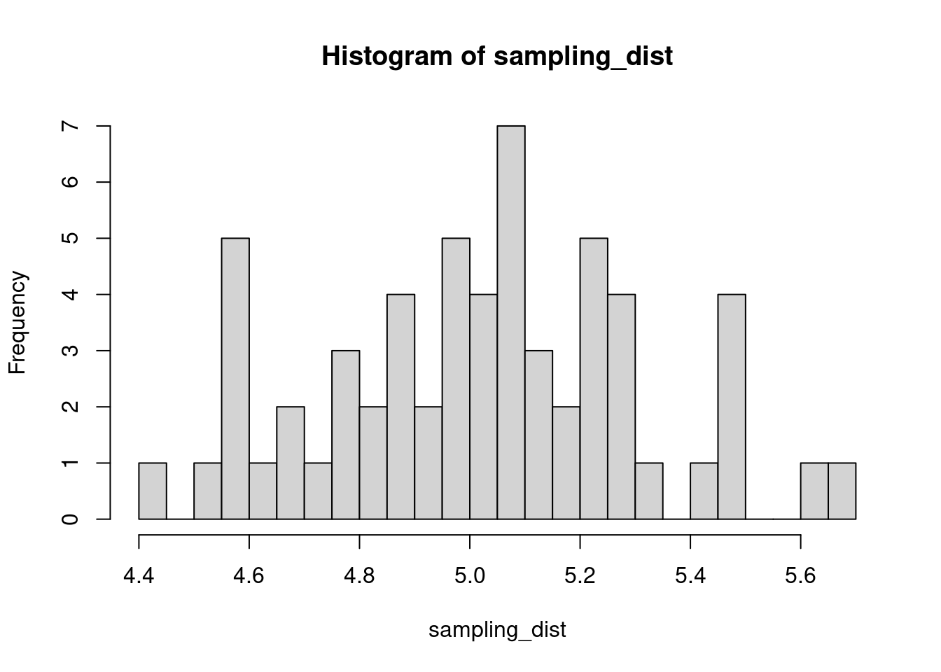
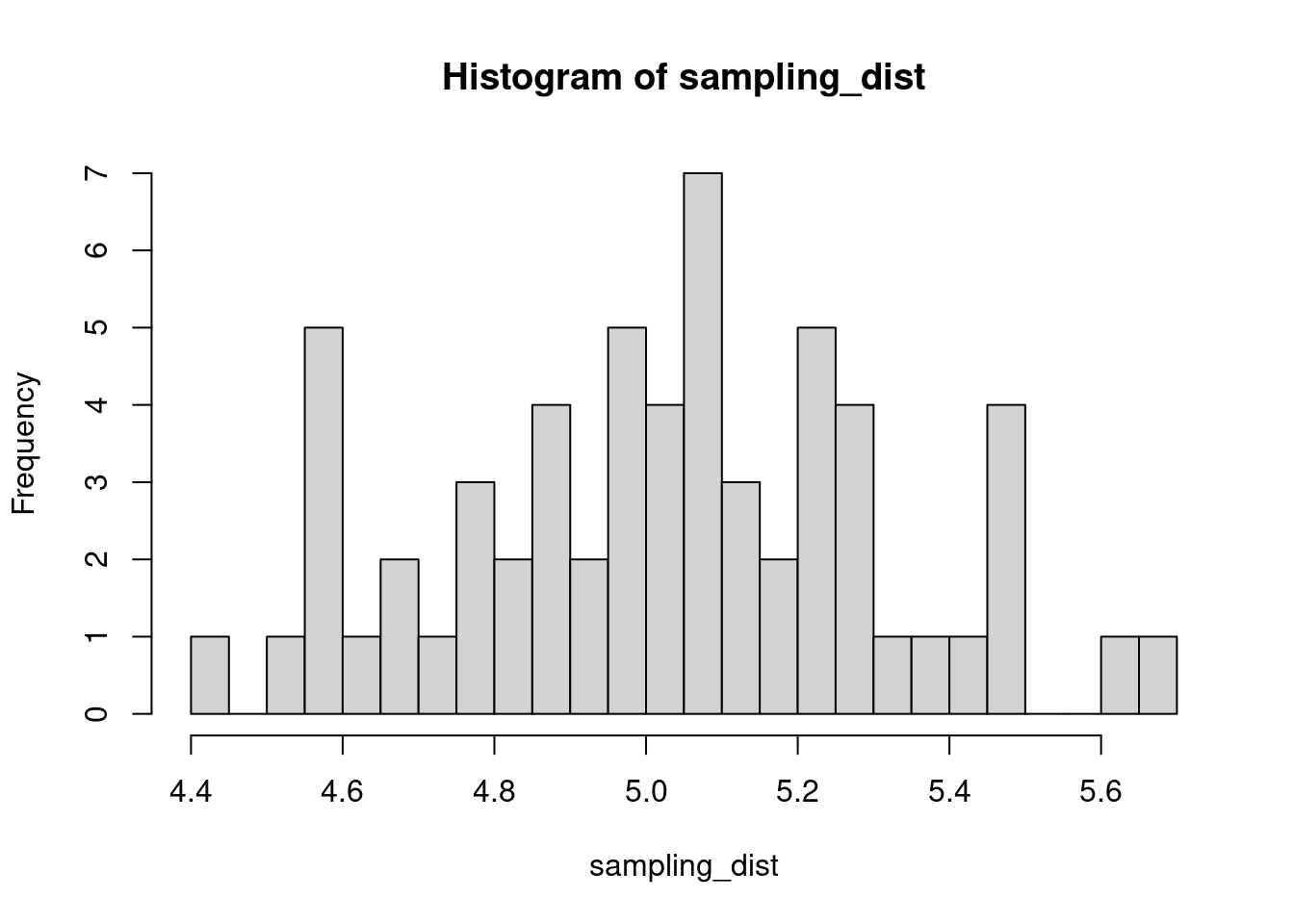
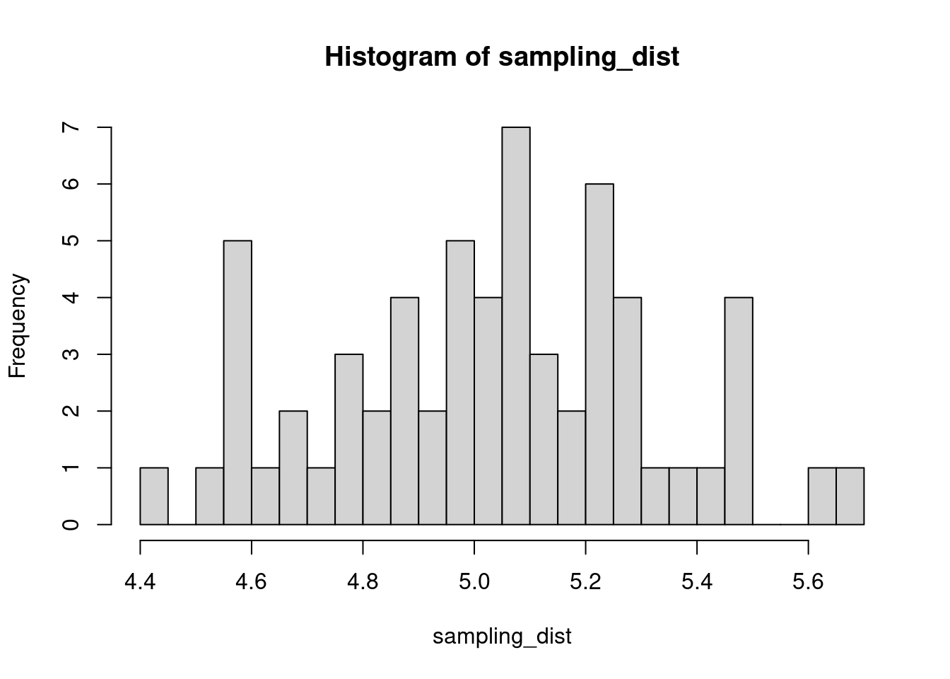
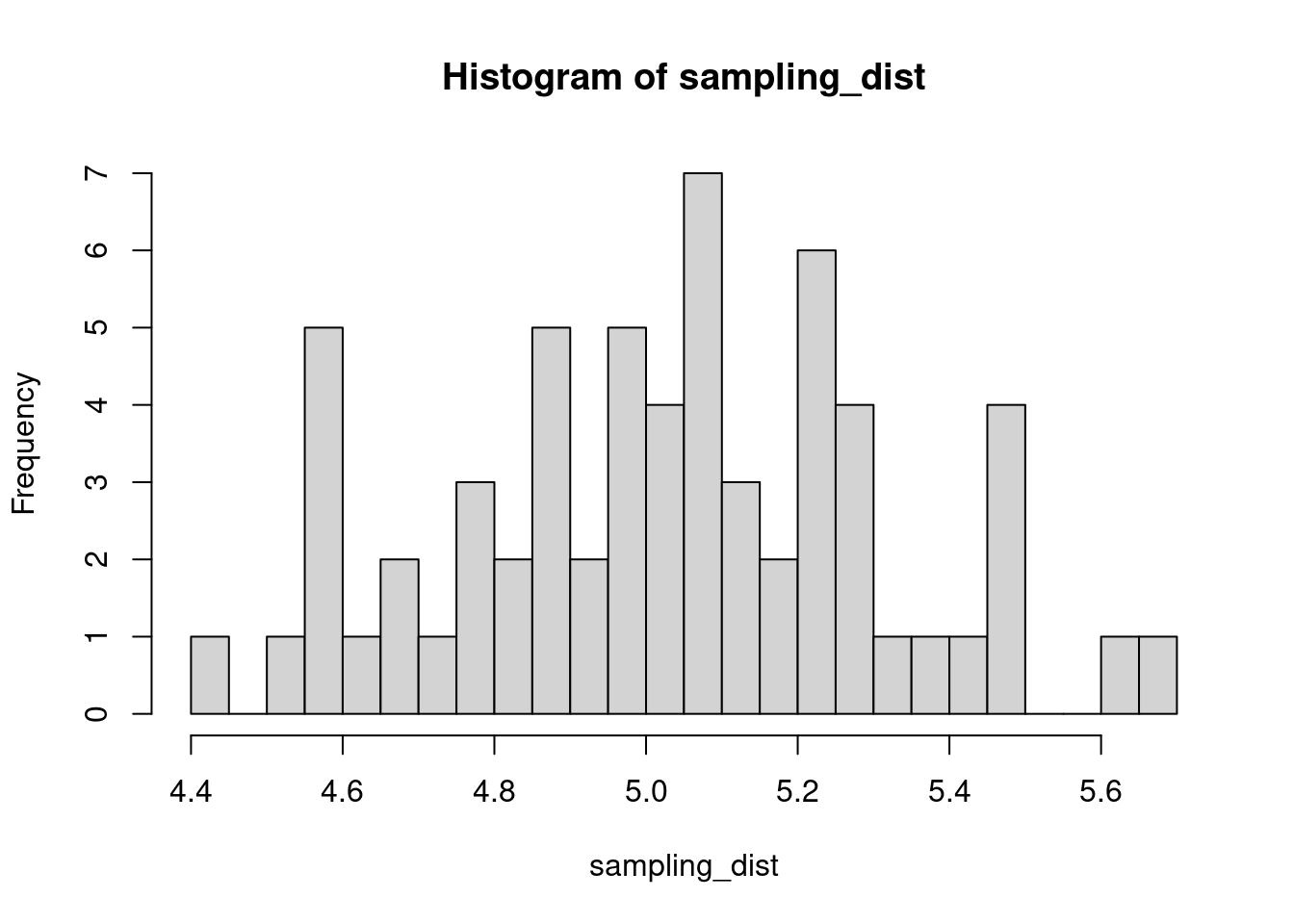
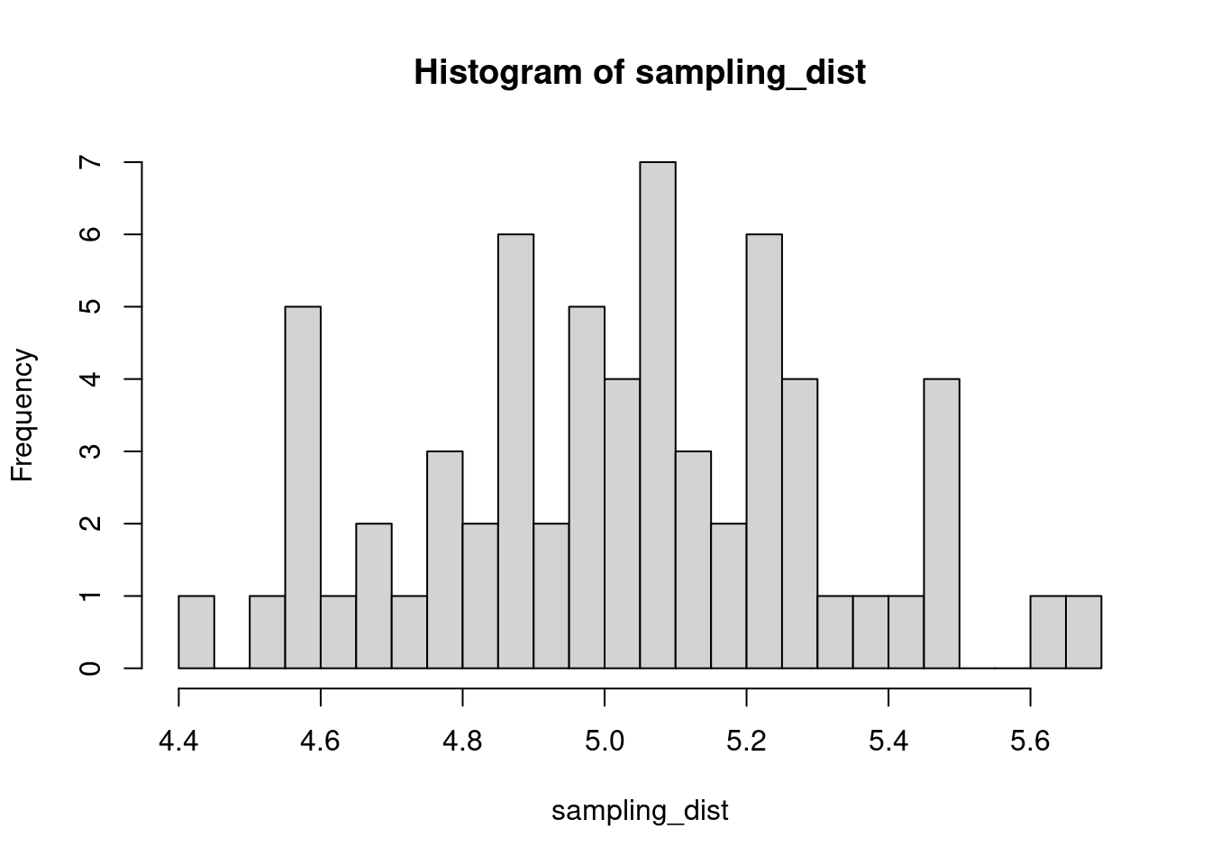
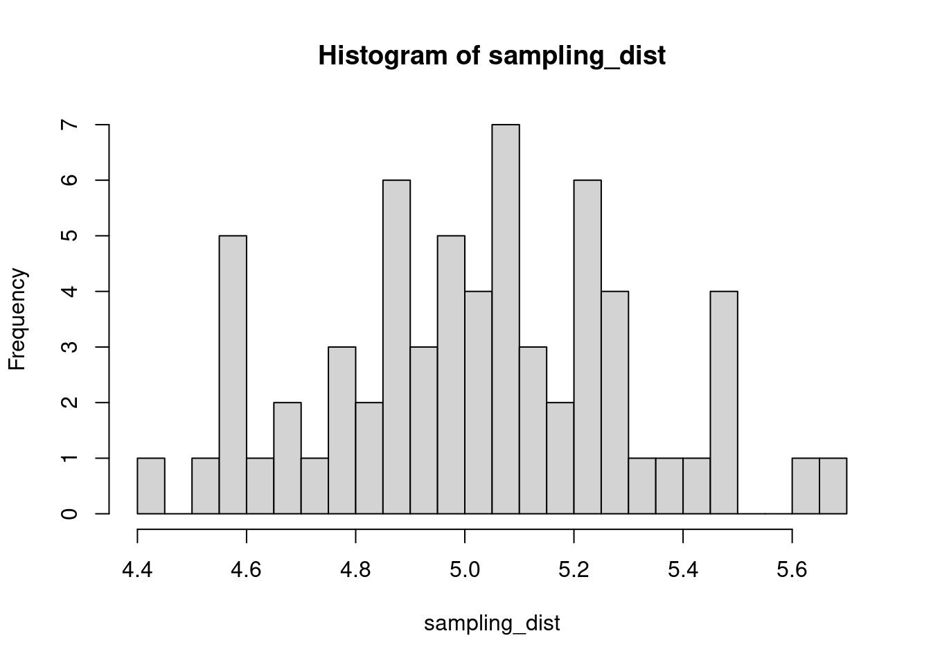
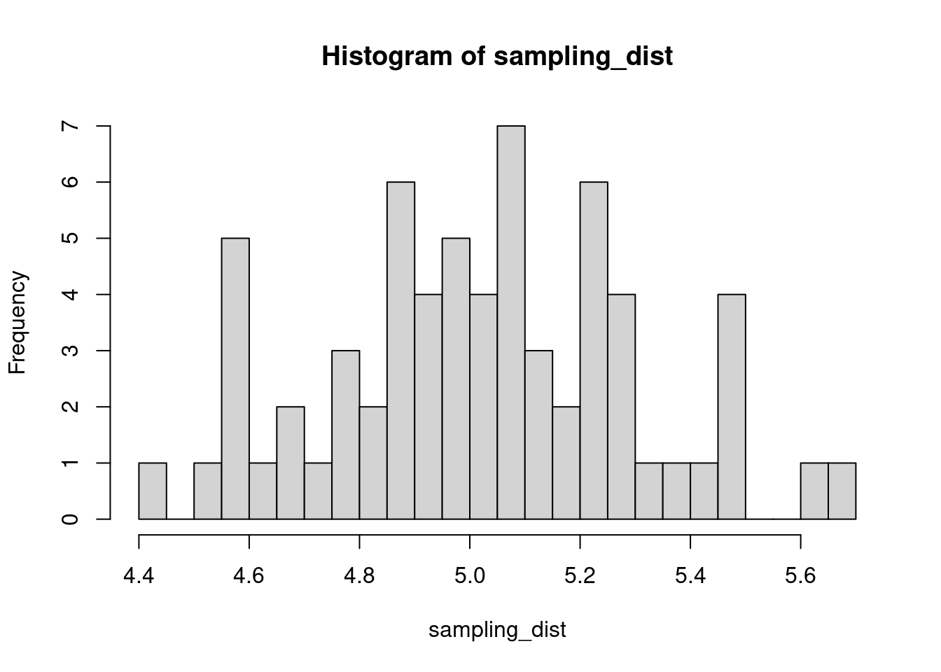
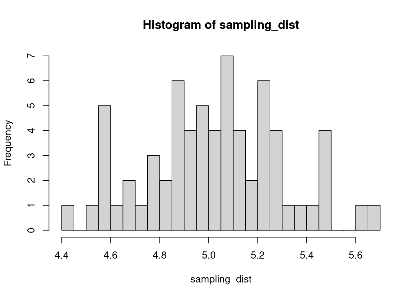
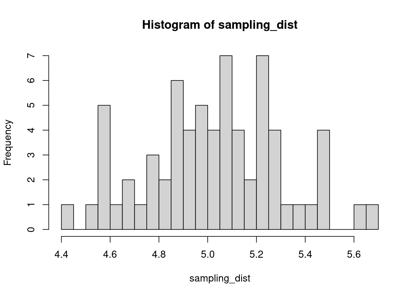
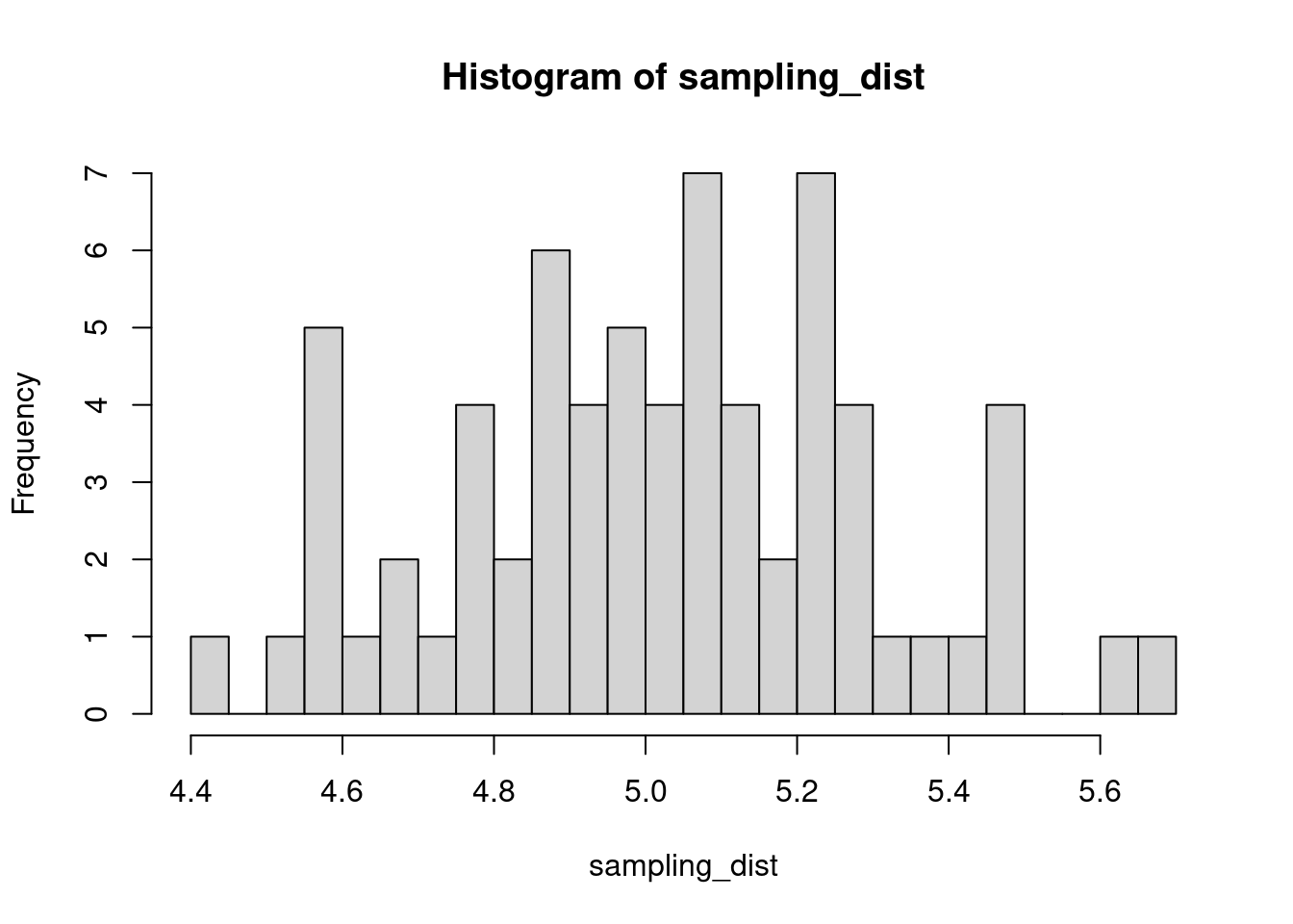

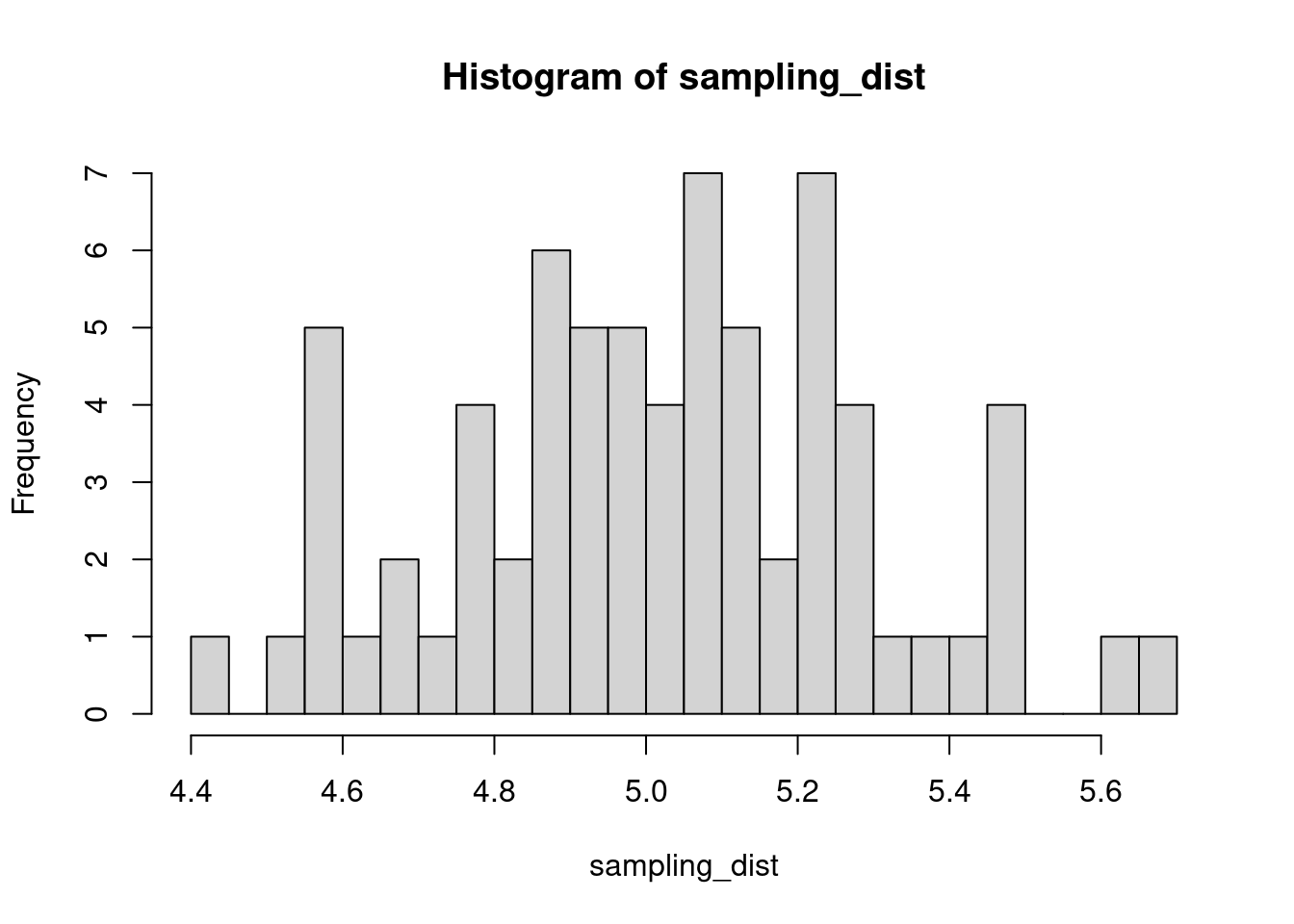
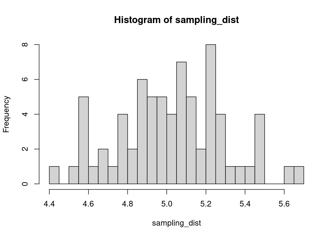
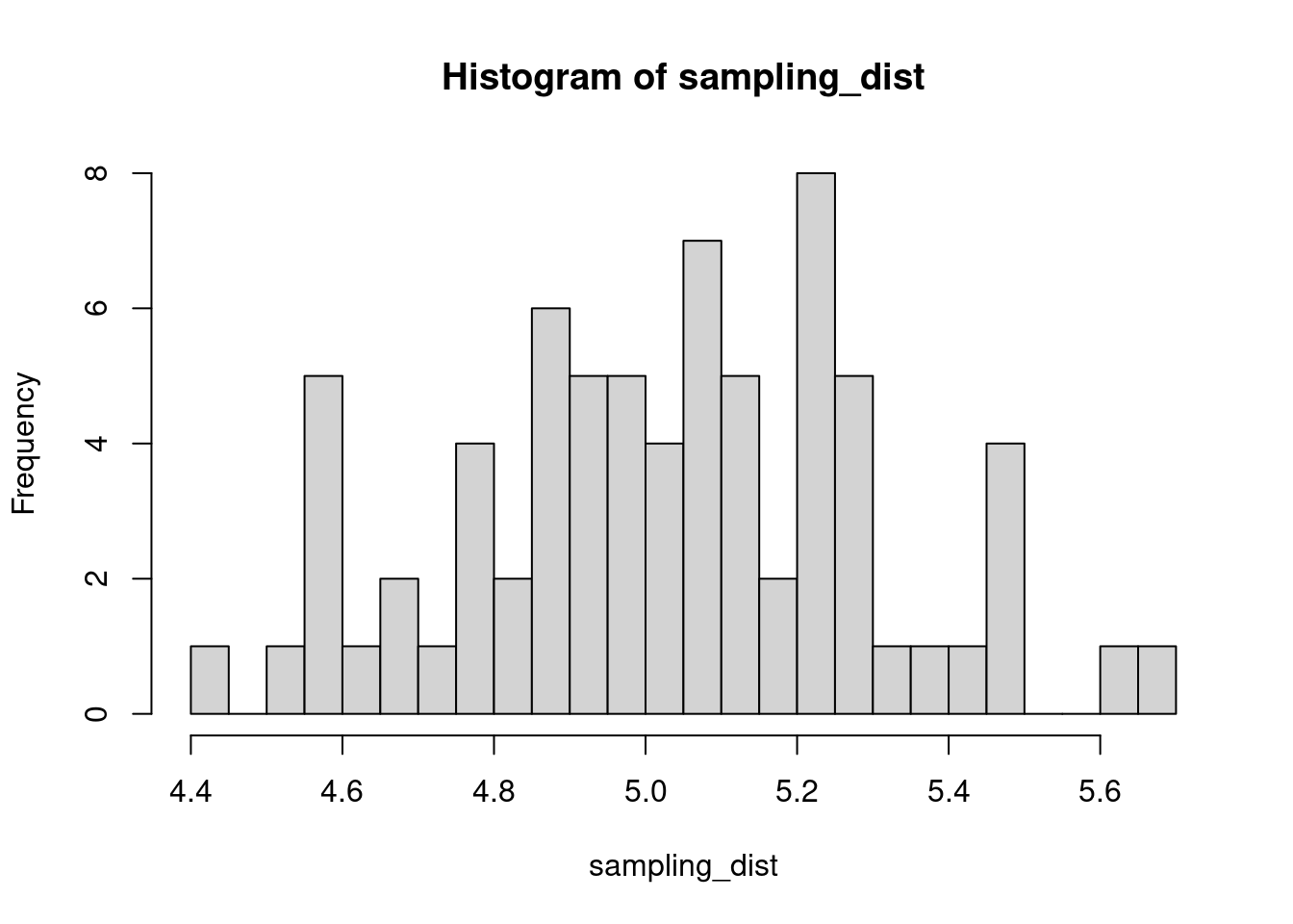
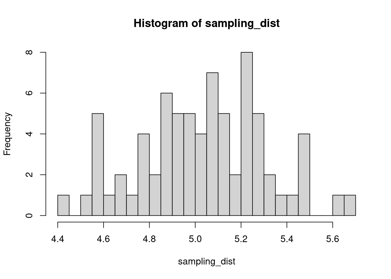
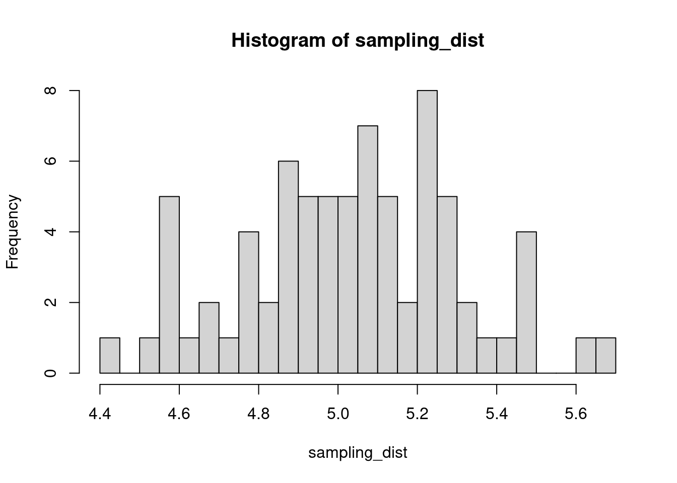
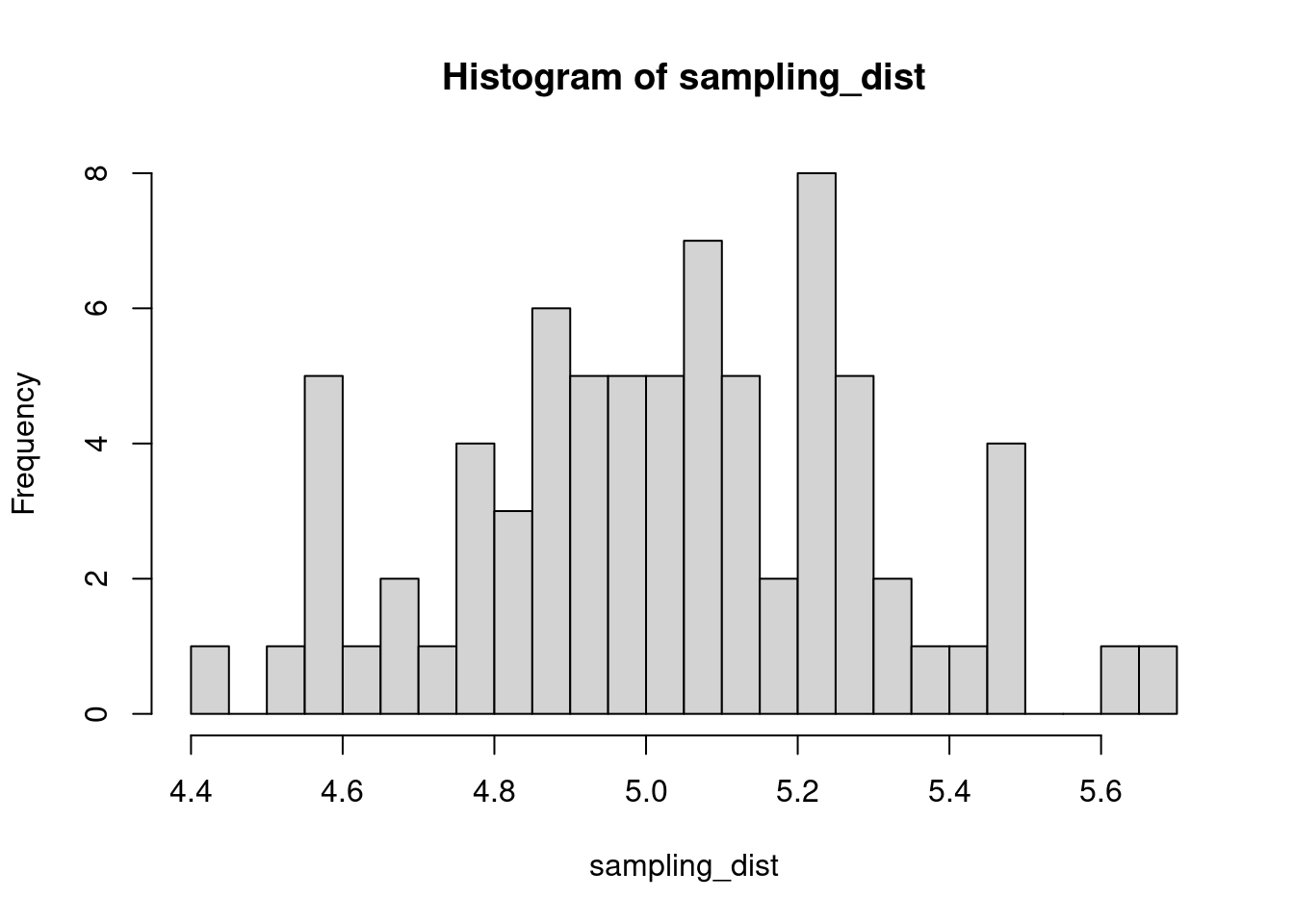


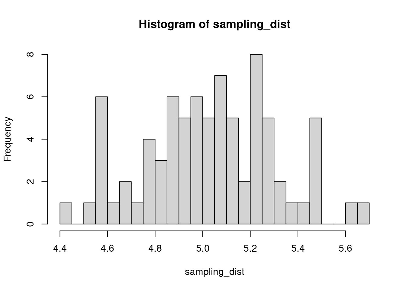
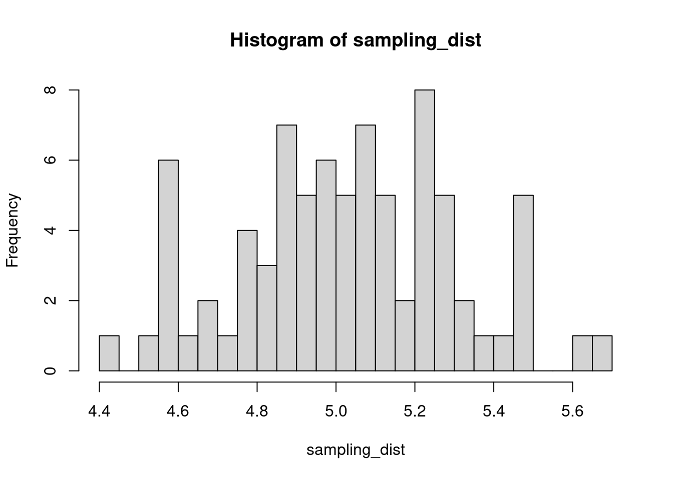
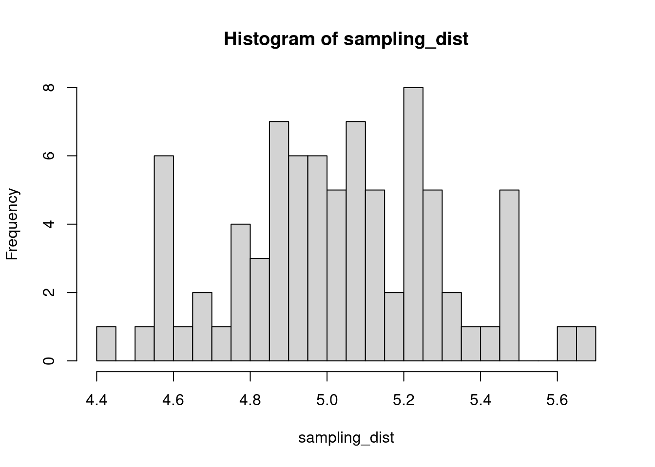
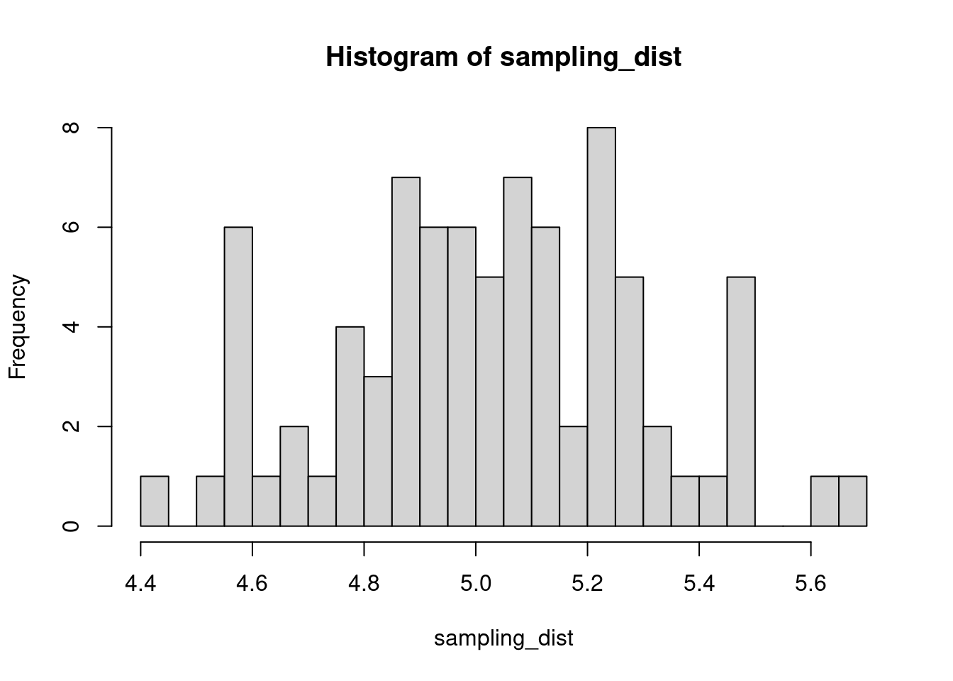
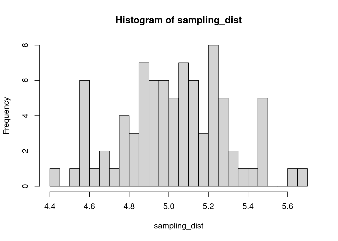
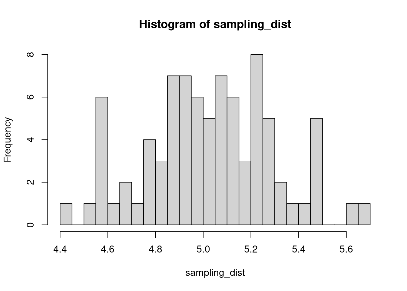
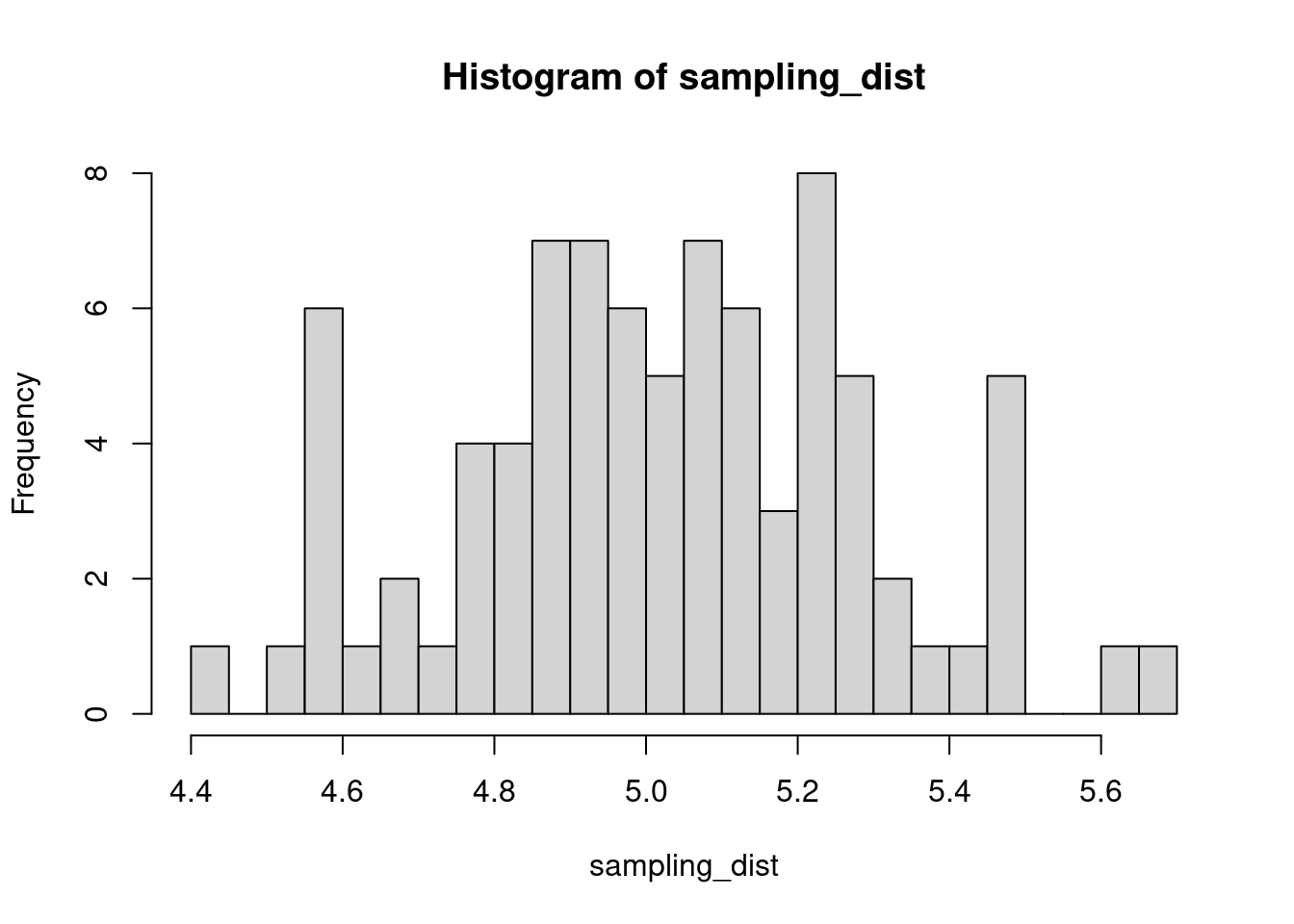
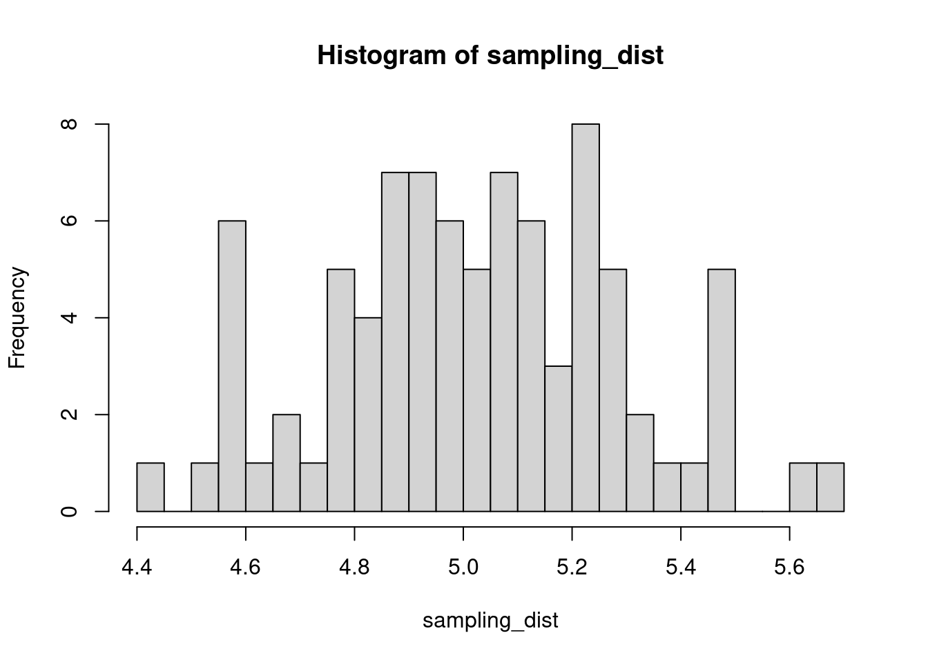
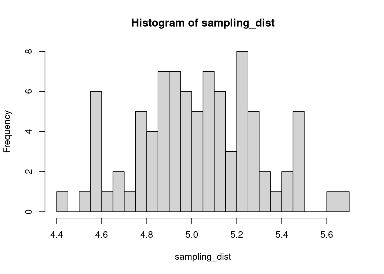

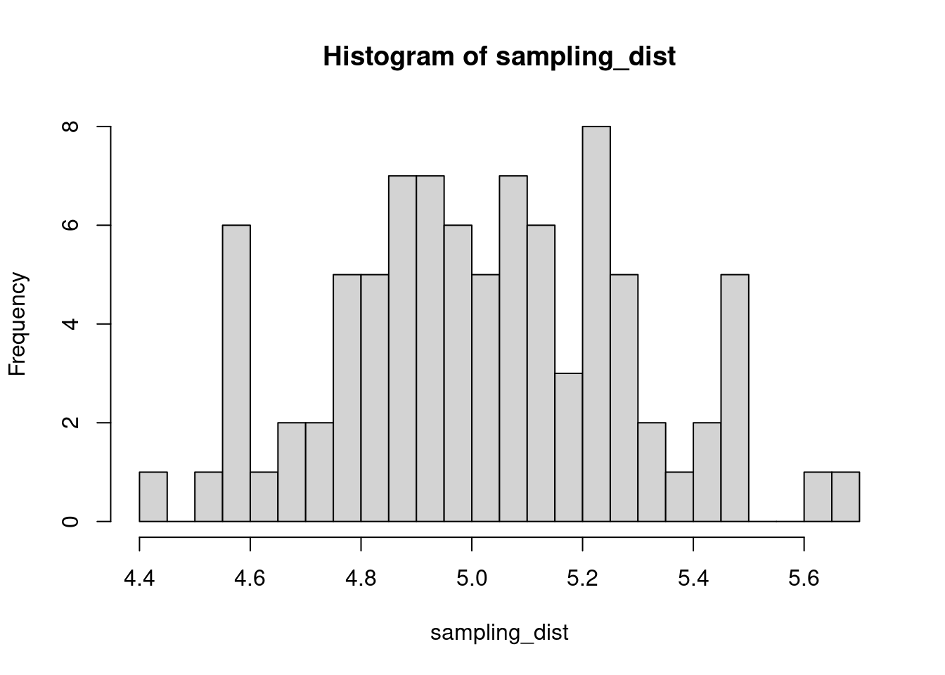
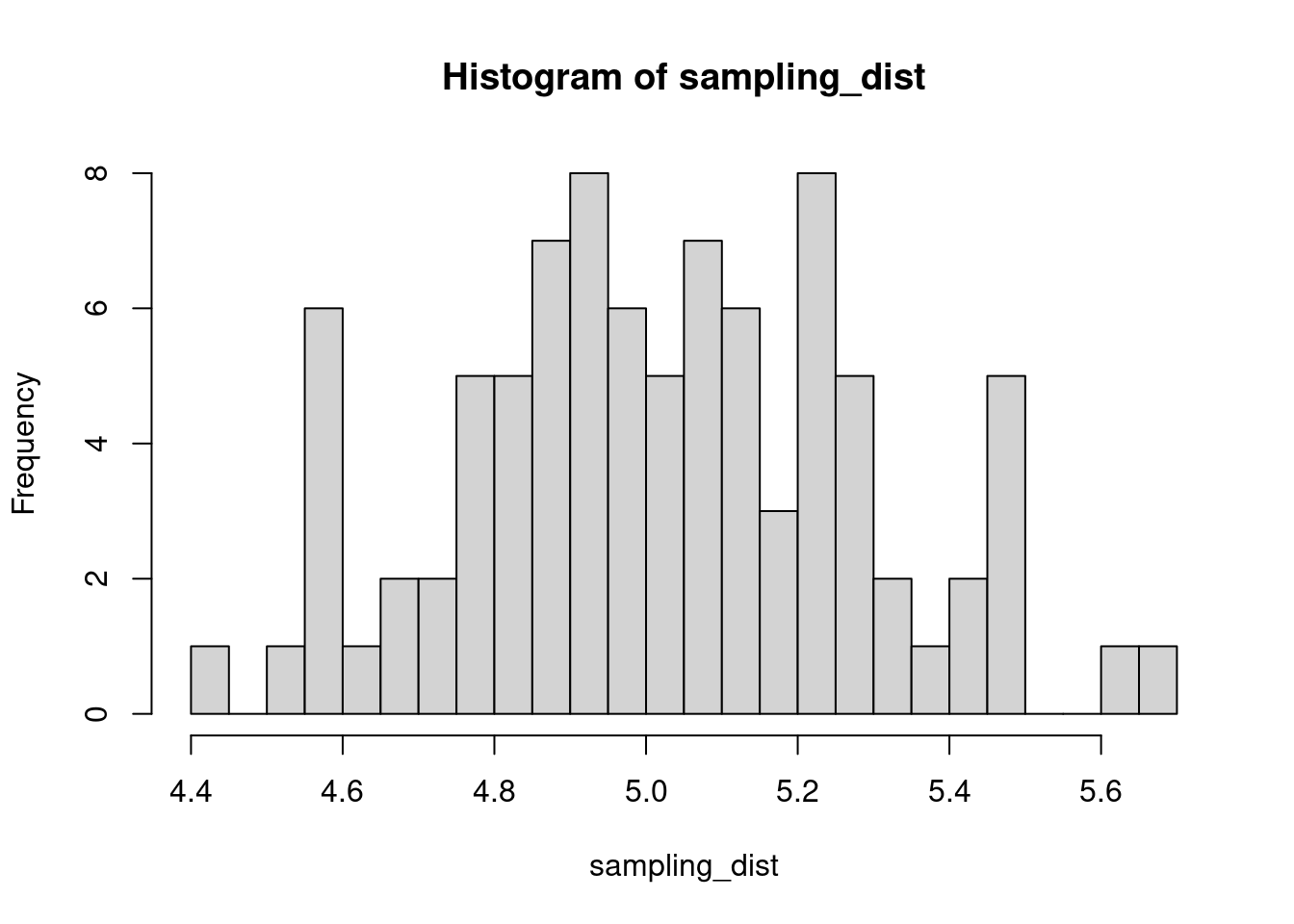
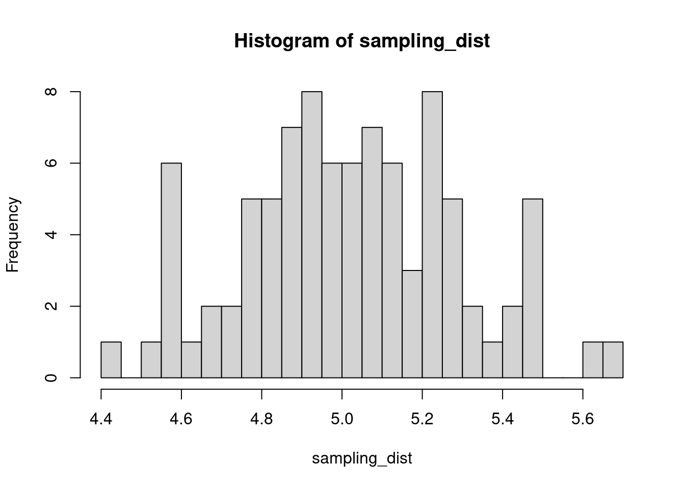
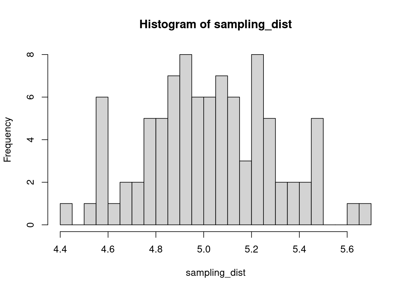
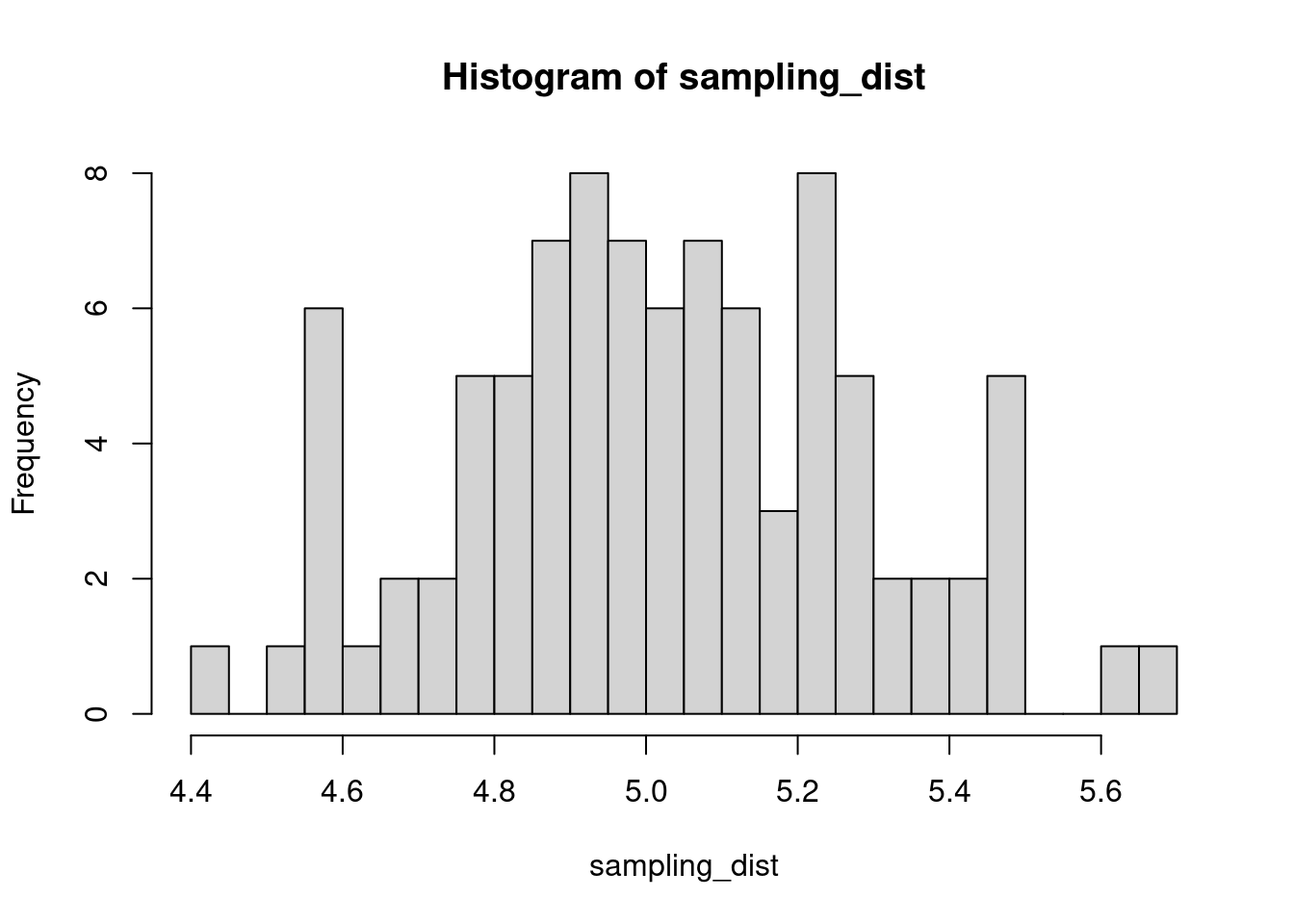
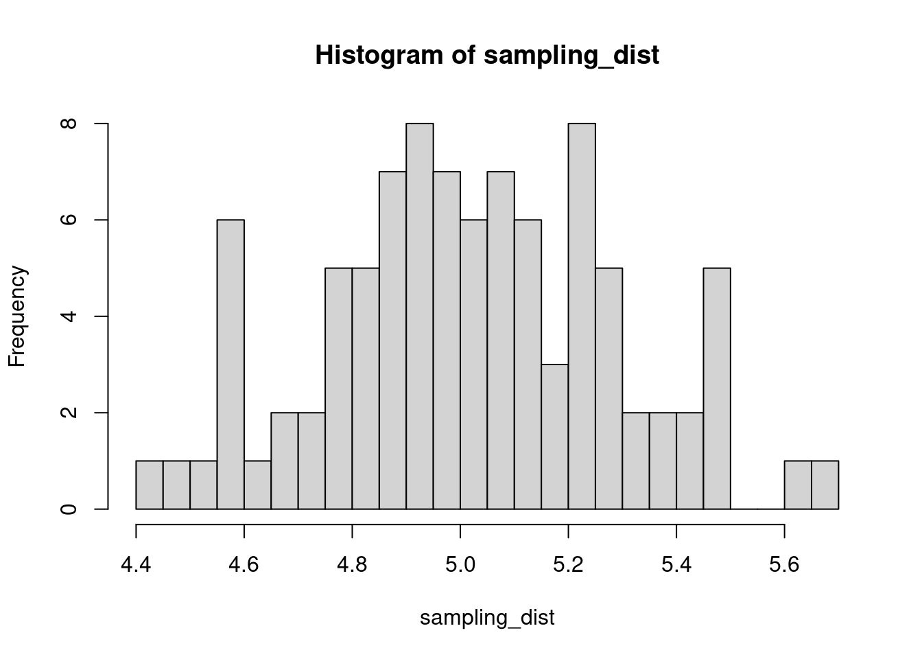
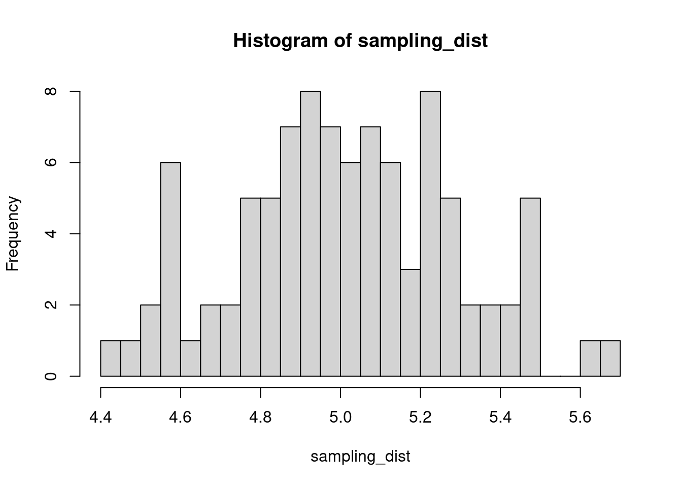
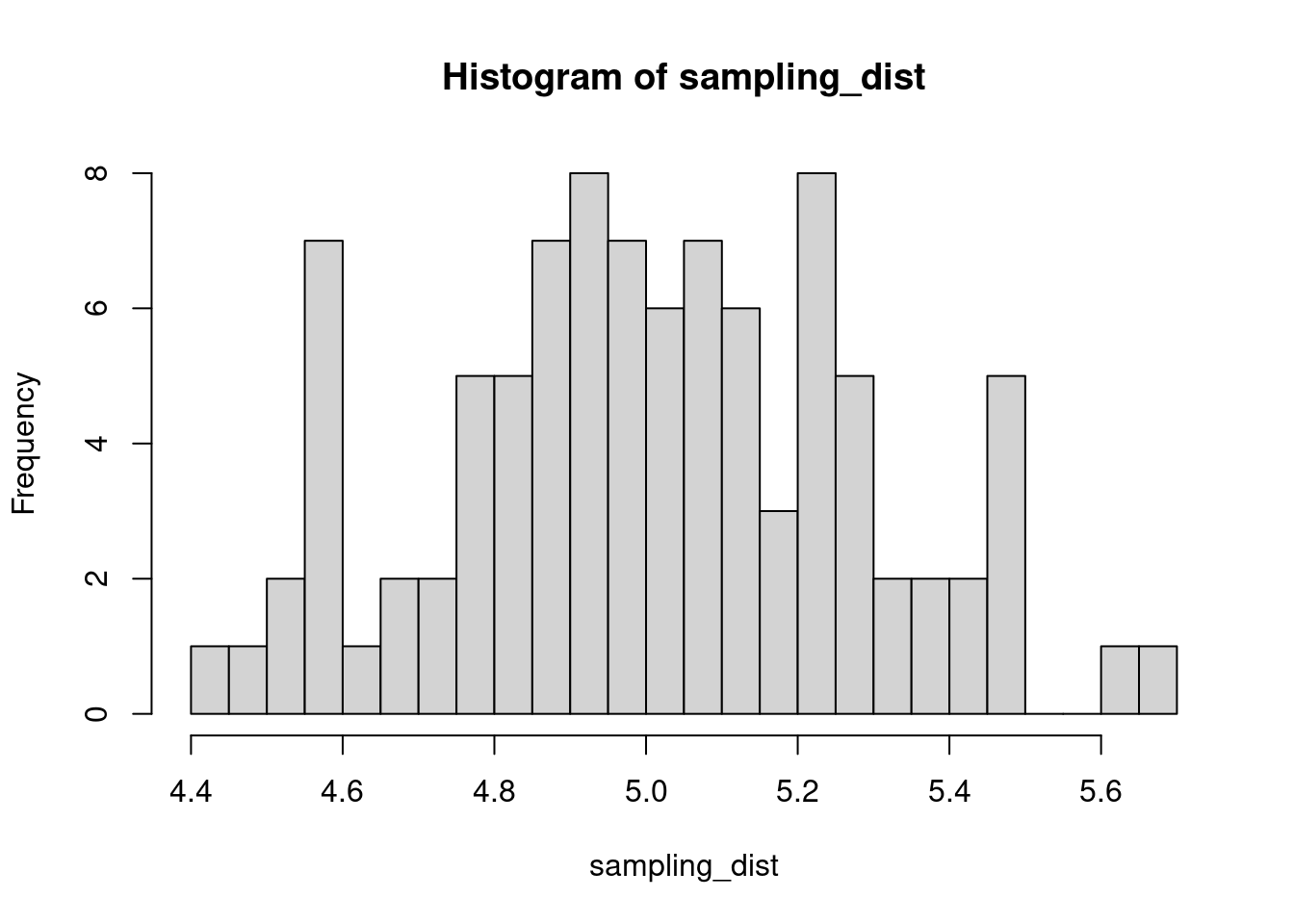
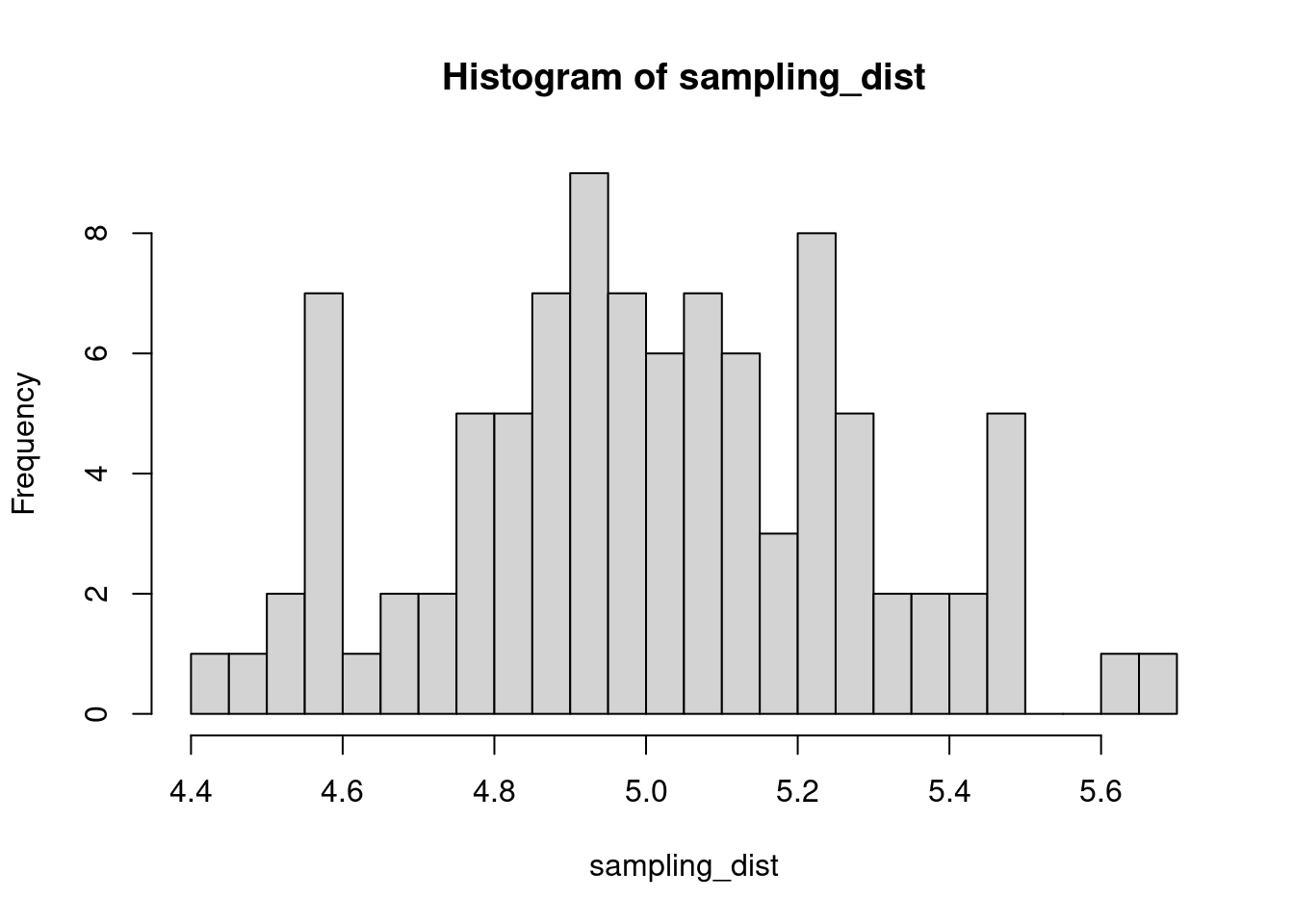
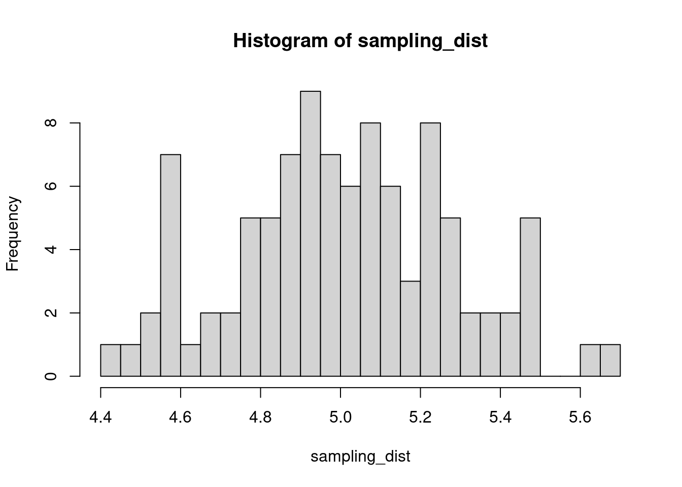
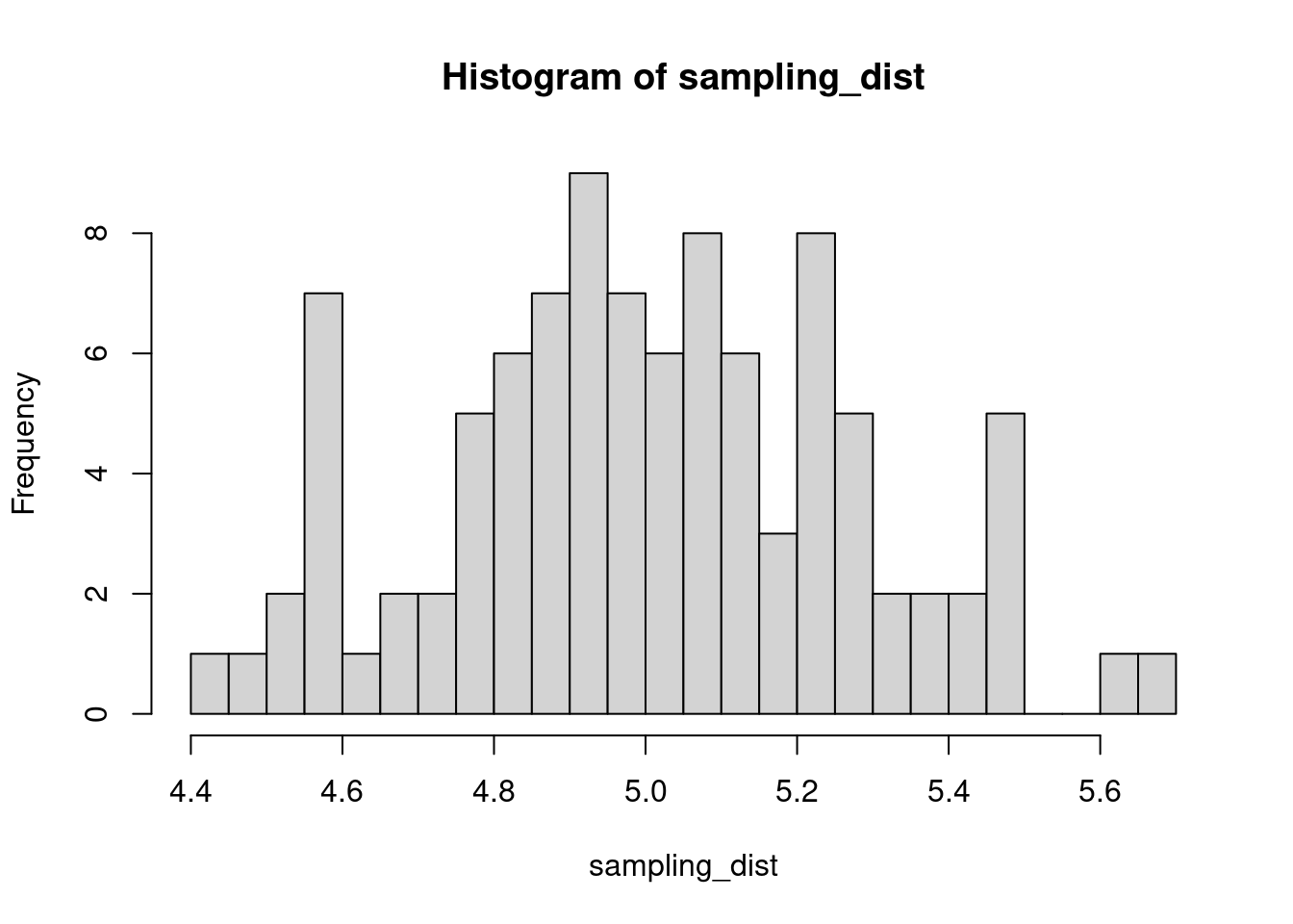
hist(sampling_dist, 20)
abline(v=mean(sampling_dist), lwd=5, col="red")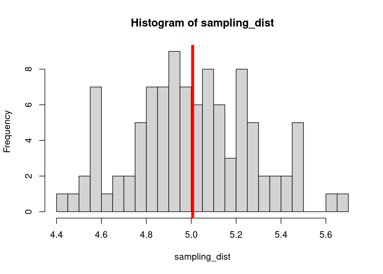
mean(sampling_dist)[1] 5.006488Now, back to models. We can add the standard error of our model estimate to our plots to indicated that there is some uncertainty in our estimated values.
# we will write this code together in class