We have so far been using a lot of built-in functions that come with R when we first install it, or that are included in packages we have installed. These functions (and packages!) were written by people (…for now, AI is coming for us all). This is why the help files vary greatly in their level of helpfulness when you use different R packages. It kinda depends on how helpful that code author was. The good news though is that if functions were written by people, that means we can also write our own functions!
The core components of a function are the arguments, and then telling R what to do with those arguments. Let’s say we want a function that adds two to any number we give it. Pointless, right?
add_two <-function(n){ output <- n +2return(output)}add_two(12.3)
[1] 14.3
add_two(c(2.7, 8, 2.4, 12))
[1] 4.7 10.0 4.4 14.0
# To answer Reese's question about why squiggly brackets:# They control the flow of information, so we are telling R that everything inside those squiggly brackets is part of the same chunk of information, and to run it all together# To answer an even more important question, why are they called squiggly brackets? They aren't. Turns out the actual name for that punctuation mark is curly brackets. I just call them squiggly because they're a bit squiggly in my mind.
7.2 I bite my thumb at thee
Functions can of course be much more complicated than that. As a mock example, we are going to build an insult generator before we get to really serious ecology (…okay fine, penguin poop) for the rest of the lesson. Let’s say we want a function that will take someone’s name and favorite number and cobble together a medieval insult for them. The arguments we will pass to the function are their name and favorite number. Then R will take that information, consult some underlying data, and behave in a predictable way to return us the response we expect.
The data we are going to use for this exercise is a spreadsheet of Shakespearean insults. It can be downloaded from https://tinyurl.com/yeastymaggot. Did I create it? No, it comes from a Python lesson by this guy. Did I pick the disgusting tinyurl handle? You betcha.
Fun fact: you can read .csv files straight from the internet. You don’t just have to read in data from your local machine.
# Read in the datadat <-read.csv("https://tinyurl.com/yeastymaggot")# One problem with this data is that it is for use in Python# Apparently those folks use both tabs *and* commas to separate data# Let's do some quick and dirty data cleaning before we start# We will combine the 'apply' function with a custom function just for this line# This is probably my most used case for the apply function: # bespoke functions that only work for one specific thing and that I don't save anywhere elsedat <-apply(dat, 2, function(x){# gsub lets us replace one string with another# in this case, a tab character with nothinggsub("\t", "", x)# note that we don't have to 'return' anything from the function # if we just want it to execute the last line which we haven't saved to an object})# now we can construct a function to bite our thumb at peoplebite_thumb <-function(first, last, n){# substr is a base R function to take a substring fl <-substr(first, 1, 1) ll <-substr(last, 1, 1)# because we need to know how to index our data fl1 <-which(letters==tolower(fl)) ll1 <-which(letters==tolower(ll))if(n>49){ n <-sample(1:49, 1) } insult1 <- dat[fl1, 1] insult2 <- dat[ll1, 2] insult3 <- dat[n, 3] output <-paste0(first, " is a ", insult1, ", ", insult2, " ", insult3)return(output)}bite_thumb("eliza", "grames", 7)
[1] "eliza is a cockered, common-kissing canker-blossom"
How long should functions be? In general, it is better to have lots of smaller functions that each do bits and pieces of what you need to accomplish, rather than one giant clunker of a function. The main reason for this is that it is easier to troubleshoot your code. You can check as you go along at specific steps to see if the output is what you expect, and can identify errors more easily. You may also realize that you only really need to run some bits of the code and not others, and it is easier to do this with more, smaller functions. You will also likely name them more sensible things. If you have a long workflow, remember that you can always nest functions within functions. Then you can create what is called a wrapper function which takes all those littler functions and wraps them all up in one neat little workflow. We will practice this with the penguin poop example.
Could you take an entire script and turn it into one giant function? Sure, but then it is likely going to be very very clunky.
At what point should you switch from just writing one long script to functions? Generally, if you find yourself doing something repetitive, it is a good idea to turn it into a function. If you need to make the same sort of calculation repeatedly but change one small thing, for example, or you keep producing the exact same type of plot and the input is the same format but different data each time, etc. Mainly, functions are good to keep your workspace neat, to save space, preserve your sanity, and make it easier to spot errors. All of these are good things when your scripts start getting especially unwieldy.
7.3 Penguin poop
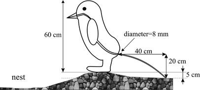
Because we are thinking about deterministic and stochastic components of linear models this week, I thought we should start with something super deterministic: physics. Specifically, the physics of how much pressure penguins must generate to expel feces from their nests. This week’s lab is inspired by Meyer-Rochow and Gal 2003 which gave science one of the most incredible figures of all time.
The greatest scientific figure of all time.
What we will be doing today is: 1) combing the paper for relevant parameters, 2) converting the paper’s equations to code, 3) replicating their analyses, and 4) evaluating how the results change when we consider a wider range of parameter estimates and incorporate stochasticity.
# First we need to establish the parameters given in the textdistance <-0.4# maximum distance reached by the poo in metersdiameter <-0.008# max diameter of an adelie penguin cloacaheight <-0.2# height (m) of the cloaca from groundtime <-0.4# estimated time it takes (seconds) for a penguin to poogravity <-10# approximate in paper; should actually be more like 9.8 m/sviscosity <-0.08# penguin poo is similar to olive oil density <-1141# presumed density of penguin pooget_radius <-function(d){ diam <- d/2return(diam)}get_velocity <-function(l,g,h){ l/sqrt(2* h/g)}get_velocity(0.4, 10, 0.2)
For loops are useful when we want to iterate across code many times, but changing values slightly. Sure, functions are already good for repetitive tasks, but what if we have created a function and we want to apply it to like 100 different options? That would take a long time! As a brief respite from penguin poo, we will switch gears for a second to children’s dances.
The Wiggles
There are apparently a lot of different versions of the lyrics to The Hokey Pokey, but apparently the US Government has an official version which we will use.
Put your right arm in, take your right arm out. Put your right arm in, and you shake it all about. Do the Hokey Pokey and you turn yourself around, that’s what it’s all about!
Put your left arm in, take your left arm out. Put your left arm in, and you shake it all about. Do the Hokey Pokey and you turn yourself around, that’s what it’s all about!
Put your right foot in, take your right foot out. Put your right foot in, and you shake it all about. Do the Hokey Pokey and you turn yourself around, that’s what it’s all about!
Put your left foot in, take your left foot out. Put your left foot in, and you shake it all about. Do the Hokey and Pokey and you turn yourself around, that’s what it’s all about!
Put your whole self in, take your whole self out. Put your whole self in, and you shake it all about. Do the Hokey and Pokey and you turn yourself around, that’s what it’s all about!
If we wanted to represent The Hokey Pokey in a for loop, the first thing we want to do is to notice repetitive patterns. First, every verse focuses on a different body part. That’s useful to note. And in each verse, we do the same set of actions in the same order: first we put the body part in, then we take it out, then we put it in, then we shake it out. And finally, we do the exact same thing after all of that, regardless of body part, and we turn ourselves around because that’s what it’s all about.
body_parts <-c("right arm", "left arm", "right foot", "left foot", "whole self")for(limb in body_parts){print(c("put", limb, "in"))print(c("take", limb, "out"))print(c("put", limb, "in"))print(c("shake", limb, "all about"))print("do the hokey pokey")}
The index that we use in a for loop remains in that loop. It will end up being saved as the very last item in the vector that is looped over. So because ‘whole self’ is the last thing that we put in during the Hokey Pokey, we now have an object named limb in our environment that is the character "whole self". Often in for loops, we use the letters i and j to represent our indices by convention, but we don’t have to.
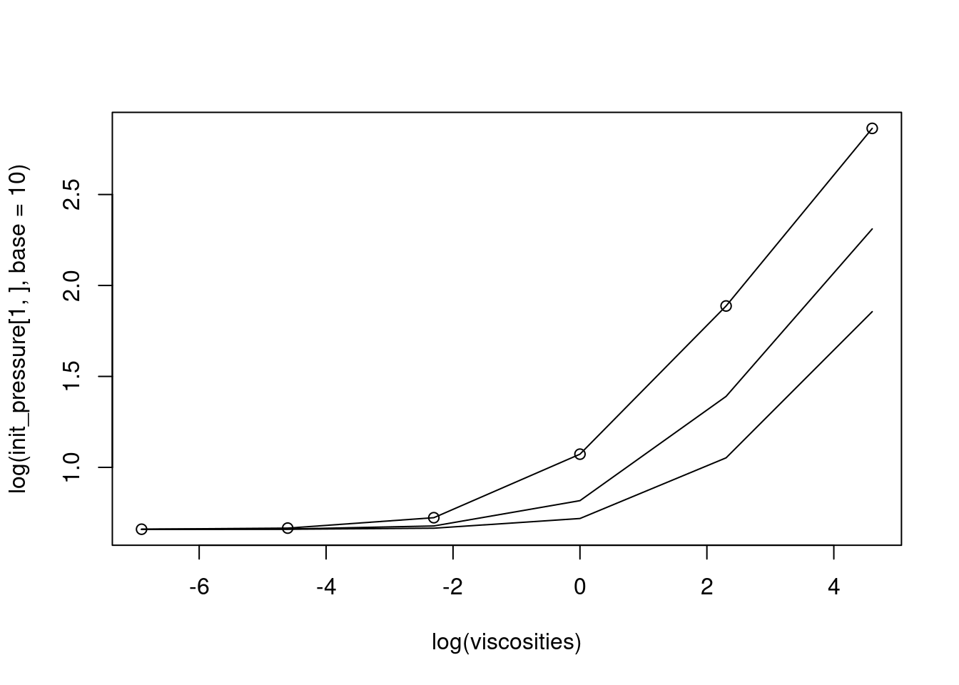
# cloacal aperture sizes for rockhoppers, adelie, and gentoo penguinsapertures <-c(0.042, 0.08, 0.138)# possible viscosities for penguin pooviscosities <-c(0.001, 0.01, 0.1, 1, 10, 100)# matrix to hold our values# note: array can be used to create a 2-dimensional array (i.e. a matrix)# I often use it because an array can have any number of dimensions# So it is more flexible than matrix()init_pressure <-array(dim=c(length(apertures), length(viscosities)))for(i in1:length(apertures)){for(j in1:length(viscosities)){ v0 <-get_velocity(distance, gravity, height) pa <-calc_pressure(density, v0)/1000 pb <-calc_hagen(nu = viscosities[j], l=distance, r=get_radius(apertures[i]), t=time)/1000 init_pressure[i,j] <- pa + pb }}plot(log(init_pressure[1,], base =10) ~log(viscosities), type="o")lines(log(init_pressure[2,], base=10) ~log(viscosities))lines(log(init_pressure[3,], base=10) ~log(viscosities))
7.5 Adding stochasticity
Because we are thinking about deterministic and stochastic components of linear models this week, let’s modify our code to incorporate some degree of uncertainty in our estimates. Realistically, penguin poop isn’t always the exact same viscosity. The authors of the paper say that the penguin poo varies from white to pink depending on how much krill they’ve eaten recently, and that the time it takes for them to excrete these different food sources varies by a number of hours. Only 9.1 hours to excrete 50% of their fecal mass if they’ve been feeding on fish, but 14.5 hours for krill. I would guess that also means there are varying levels of penguin poo viscosity. While we’re at it, I would also guess that the maximum diameter of each penguin cloaca varies quite a bit too, as does the height they are from the ground on the edge of their nest, etc.
# note: we will code this section together in lab
7.6 While loops
For loops have a fixed number of iterations. ‘while’ loops on the other hand will run until a specific condition is met. This is dangerous, because that means they could literally keep running forever if the condition is never met. Think about all the possible loopholes, because otherwise you can run into problems with a ‘while’ loops. When would you want to use them? Honestly, not very often. But they are useful to know about I suppose.